DDPM: Diffusion Model Background

The introduction and background of DDPM did not explain diffusion basics sufficiently for me, so I used several blogs to write this separate overview.

0. Abstract

This paper proposes diffusion probabilistic models, latent-variable models inspired by nonequilibrium thermodynamics that perform high-quality image synthesis. It uses a connection between diffusion and denoising score matching with Langevin dynamics.

1. Introduction

• The paper presents advances in diffusion probabilistic models.

• A diffusion model gradually adds noise to data or reconstructs data from noise to generate data.

• The figure below summarizes this. $x_0$ is real data, $x_T$ is final noise, and intermediate $x_t$ denotes latent variables containing noisy data.

• The goal is to find $p_{\theta}(x_0) = \int p_{\theta}(x_{0:T}) dx_{1:T}$. Here, $p_{\theta}(x_{0:T})$ is the reverse process and $x_1,…,x_T$ consists of latents with the same dimensionality as $x_0 \sim q(x_0)$.

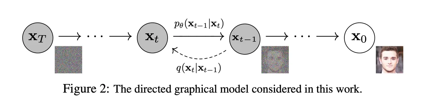
• First, the forward process $q(x_{t}|x_{t-1})$ gradually adds noise, moving right to left in the figure. Learning a reverse process $p_{\theta}(x_{t-1}|x_t)$ that estimates the inverse of this forward process teaches reconstruction of $data(x_0)$ from $noise(x_T)$.

• Using this reverse process, the model can generate images, text, graphs, and other desired data from random noise.

2. Background

(1) Forward Diffusion Process (q)

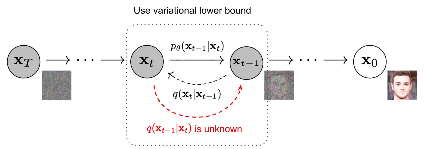
• The forward diffusion process, q, is a Markov chain that $data(x_0)$adds noise from the initial data to final noise $noise(x_T)$. This runs opposite to sampling. We need its distribution because reverse-process learning uses information from the forward process.

• Noise is scaled according to the variance schedule $\{\beta_t \in (0,1)\}_{t=1}^{T}$ before being added.
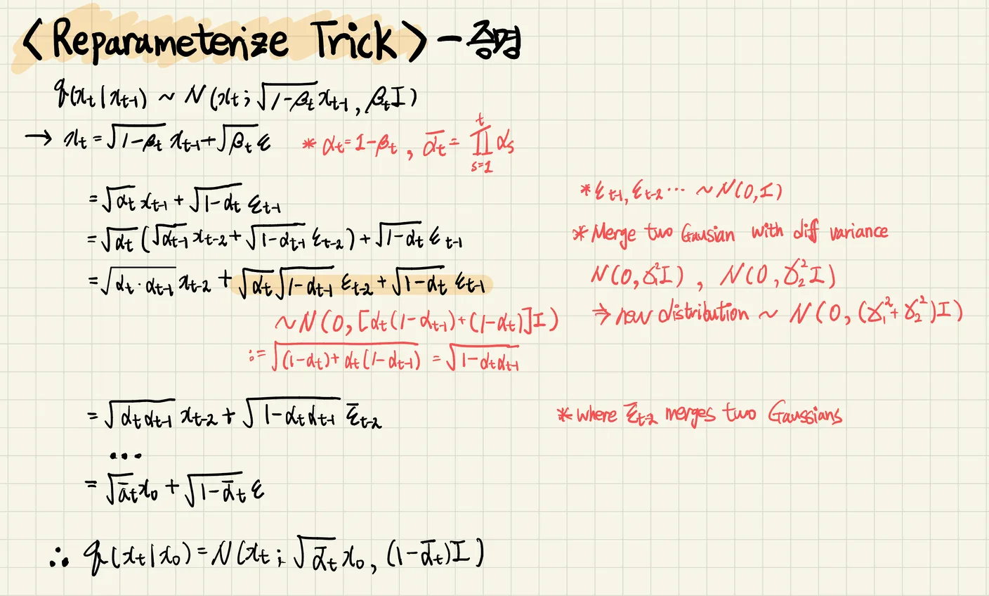
• Each step samples a Gaussian through reparameterization. Scaling by $\sqrt{1-\beta_t}$, rather than merely adding noise, prevents variance from diverging.
• Keeping variance near unit scale maintains it at a controlled level throughout the forward and reverse processes.
$$x_t = \sqrt{1-\beta_t}\ x_{t-1} + \beta_t * \epsilon \\ (\sqrt{1-\beta_t})^2 + \beta_t = 1$$
• The schedule could be learnable, but experiments found little difference from fixed values, so it is kept constant.
• Its value is small when data still resembles an image and increases as it approaches a Gaussian, rising linearly from 10^-4 to 0.02.

• We can produce $x_t$ from $x_0$ by taking t sequential steps, or do it directly.
• Recursively rearranging the equation gives the distribution of $x_t$ for given data $x_0$ as follows.
$$a_t := 1-\beta_t \ and \ \bar{\alpha_t} := \prod_{s=1}^{t}\alpha_s \\ q(x_t|x_0) = \mathcal{N}(x_t;\sqrt{\bar{\alpha_t}}x_0,\ (1-\bar{\alpha_t})\mathrm{I})$$
• Training one step at a time uses too much memory and computation. Directly producing the noisy sample lets us calculate the loss and take an expectation over t. Since training uses stochastic gradients, this is sufficient.

(2) Reverse Diffusion Process (p)

• The reverse diffusion process p $noise(x_T)$ reconstructs $data(x_0)$ from noise.

• Modeling this process is essential because it ultimately generates data from random noise, but determining the actual process is difficult.

We want to know $q(x_{t-1}|x_t)$, but it is difficult to obtain.

• We therefore approximate it with $pθ$, a Markov chain using Gaussian transitions, expressed below.

• At each step, the Gaussian mean $\mu_θ$ and standard deviation $\sum_θ$ are parameters to learn. The starting noise distribution is defined as the simplest standard normal distribution below.

(3) Objective Function (Loss)

• Now that we understand forward and reverse processes, let us examine training to estimate the parameters of $p_\theta$.

• Our goal is to find the true data distribution $p_\theta(x_0)$, so we want to maximize likelihood, or minimize negative log-likelihood. This is expressed below.

• The third equality in the training loss holds because both processes are Markov chains: it follows from the Markov property.
Markov property

Given the current state, the probability of the next state is independent of how we reached the current state.

• Finally, rearrange the expression into KL divergences between Gaussian distributions to make computation easier.

• Let us examine each term using the equations introduced earlier.
• LT: The distribution difference between $noise(x_T)$ generated by p and $noise(x_T)$ generated by $q$ given data $x_0$.
$q(x_T|x_0)$ and $p(x_T)$

(1) $q(x_t|x_0) = \mathcal{N}(x_t;\sqrt{\bar{\alpha_t}}x_0,\ (1-\bar{\alpha_t})\mathrm{I})$

(2) $p(x_T) = \mathcal{N} (x_T;0,\mathrm{I})$

• Lt−1: The difference between the reverse and forward transition distributions p and q. Training makes them as similar as possible.
$q(x_{t-1}|x_t, x_0)$ and $p_{\theta}(x_{t-1}|x_t)$

(1) $q(x_{t-1}|x_t)$ is unknown, but $q(x_{t-1}|x_t, x_0)$ is known.

By Bayes' rule, using posterior and prior! $P(x_{t-1}|x_t) = {P(x_t|x_{t-1}) P(x_{t-1}) \over P(x_t)}$

$q(x_{t-1}|x_t, x_0) = q(x_t|x_{t-1}, x_0){q(x_{t-1}|x_0)\over q(x_t|x_0)}$

$\therefore reverse\ conditional \ probability,\\ \ q(x_{t-1}|x_t, x_0) = N(x_{t-1}; \tilde{\mu}(x_t,x_0), \tilde{\beta}t\mathrm{I}) \\ \tilde{\mu}t(x_t,x_0) = \sqrt{\bar{\alpha}{t-1}\over1-\bar{\alpha_t}}\beta_tx_0 \ + {\sqrt{\alpha_t}(1-\bar{\alpha}{t-1})\over 1-\bar{\alpha}t}x_t, \ \tilde{\beta_t} = {(1-\bar{\alpha}{t-1})\over 1-\bar{\alpha}_t}$

(2) $p_{\theta}(x_{t-1}|x_t):=\mathcal{N}(x_{t-1};\mu_{\theta}(x_t,t),\ \sum_\theta (x_t,t))$

• L0: The likelihood of estimating data x0 from latent x1, which training maximizes.
 

View proof

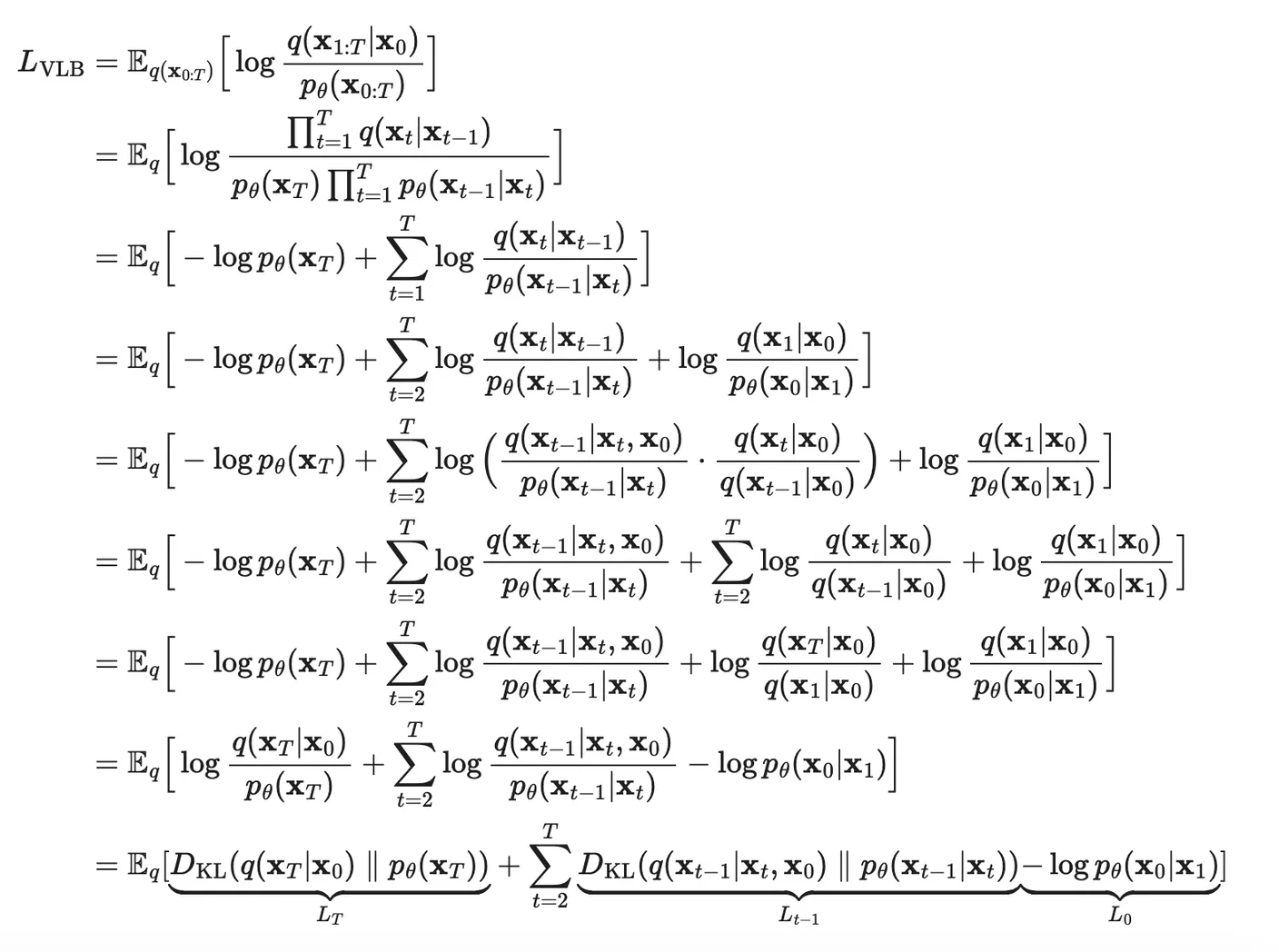
• Ultimately, the training loss is easily computed as KL divergence between Gaussian distributions.

References

1. Ho, J., Jain, A., & Abbeel, P. (2020). Denoising diffusion probabilistic models.  Advances in Neural Information Processing Systems, 33, 6840-6851.

2. https://lilianweng.github.io/posts/2021-07-11-diffusion-models/

3. https://happy-jihye.github.io/diffusion/diffusion-1/

4. https://process-mining.tistory.com/182