DreamMat: High-quality PBR Material Generation with Geometry- and Light-aware Diffusion Models

DreamMat: High-quality PBR Material Generation with Geometry- and Light-aware Diffusion Models

Paper: https://arxiv.org/abs/2405.17176 Project Page: https://zzzyuqing.github.io/dreammat.github.io/ Github: https://github.com/zzzyuqing/DreamMat

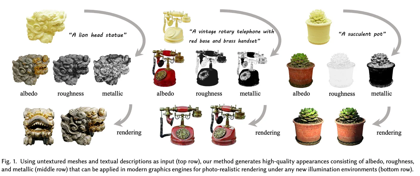
My thoughts on the paper

• A useful paper for thinking about PBR.

• Strengths
• Shows substantial thought about the problem of PBR material generation.
• Includes considerable classical graphics knowledge, such as BRDF, SVBRDF, and the rendering pipeline.
• The authors seem to have thought carefully about PBR representation too.
• Learning material parameters and sampling them to generate textures should avoid occlusion-related gaps.

• Weaknesses
• I need to run the code to assess quality, but generation takes twenty minutes.
• The main contribution may amount to training a light ControlNet.
• The representation section mostly describes existing knowledge.
• The CSD loss also seems to supplement an existing method with effective negative-prompt keywords.
• I wonder whether methods using diffusion as a loss, such as SDS and CSD, will remain mainstream.
• Quality: Oversaturation and unnatural results may be difficult to eliminate.
• Speed: Since optimization is required, reducing runtime may be difficult.

Abstract

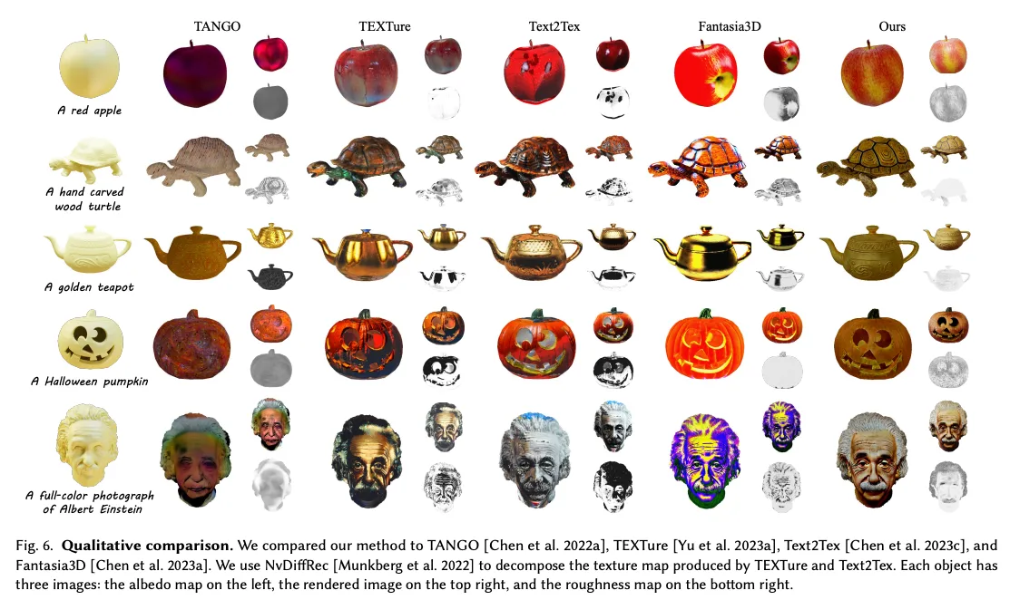
Advances in 2D diffusion now allow appearance, or textures, to be generated for raw meshes. But RGB textures often bake in unwanted shading. Physically based rendering materials would be a more ideal solution, yet existing methods struggle with inaccurate material decomposition, such as shading left in albedo. DreamMat generates PBR materials from text, addressing the difficulty caused by 2D diffusion models learning only final shaded colors. A newly fine-tuned, light-aware diffusion model removes shading effects from albedo.

1. Introduction

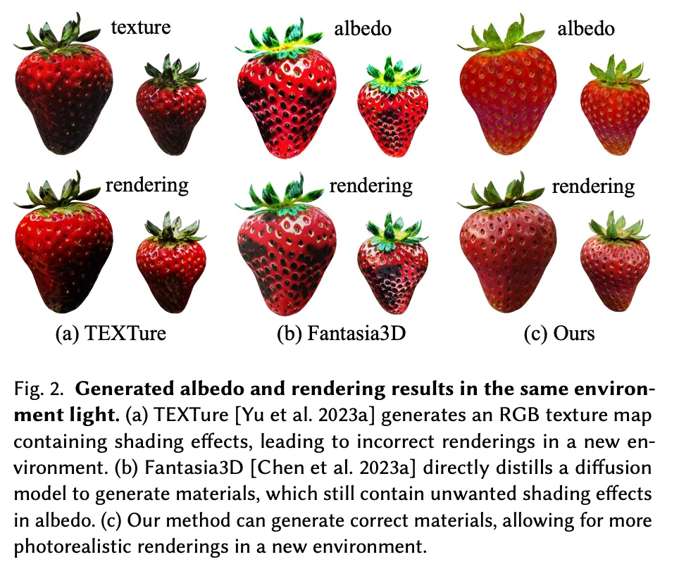
Methods such as TEXTure do not support PBR. Fantasia3D does, but leaves shading in albedo. Directly training a material-generation network is difficult because high-quality 3D PBR datasets are scarce. Training-free alternatives such as Fantasia3D distill 2D diffusion models to decompose generated appearance into materials, but still leave shading behind. Material decomposition is ill-posed: there is no single unique answer.

The paper analyzes this ill-posedness within diffusion distillation. Diffusion models are trained to generate natural RGB images, whose shading reflects unknown environment lighting and materials. Fantasia3D fixes a single environment light during distillation, but the generated image may not match that lighting. The paper attributes inaccurate material estimates to this inconsistency.

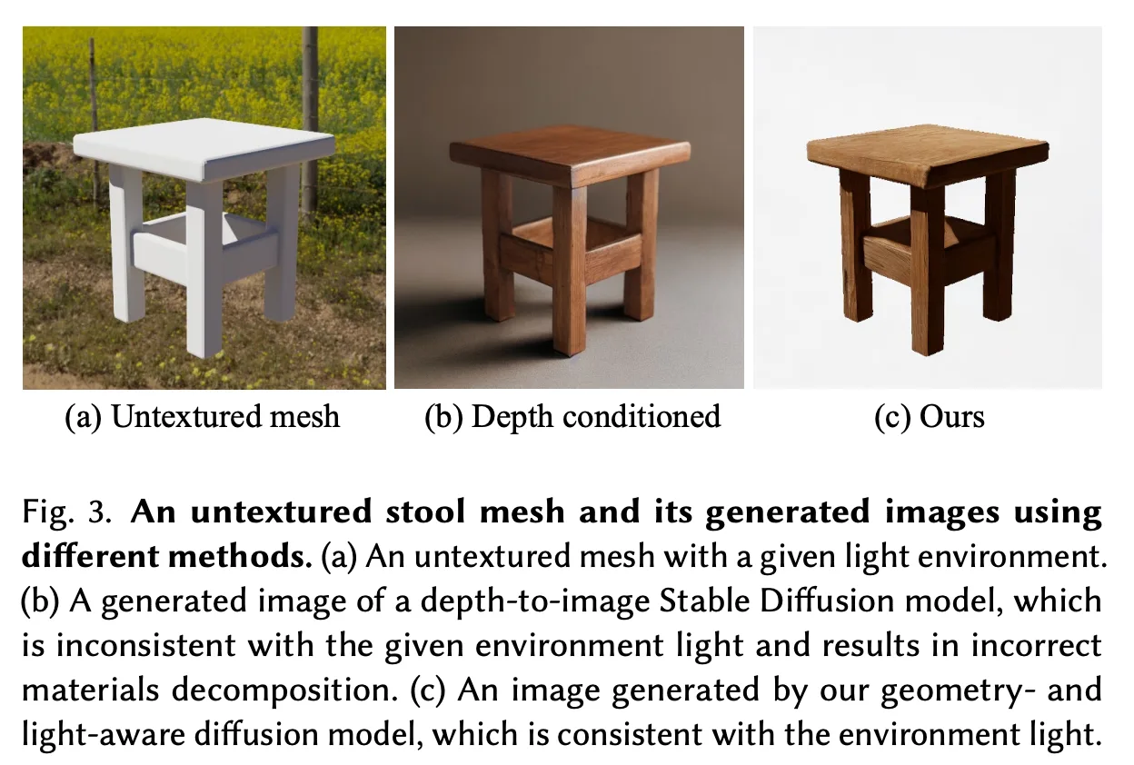
DreamMat proposes two key ideas. First, it chooses random HDR images as environment lights during distillation, encouraging the model to focus on estimating object materials. Second, a geometry- and light-aware diffusion model is trained to generate images consistent with given lighting. In Figure 3(c), generated shading matches the shading on the untextured mesh. Distilling this model enables more accurate material generation. The contributions are:

• A geometry- and light-aware diffusion model.

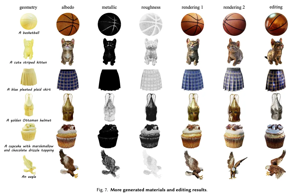
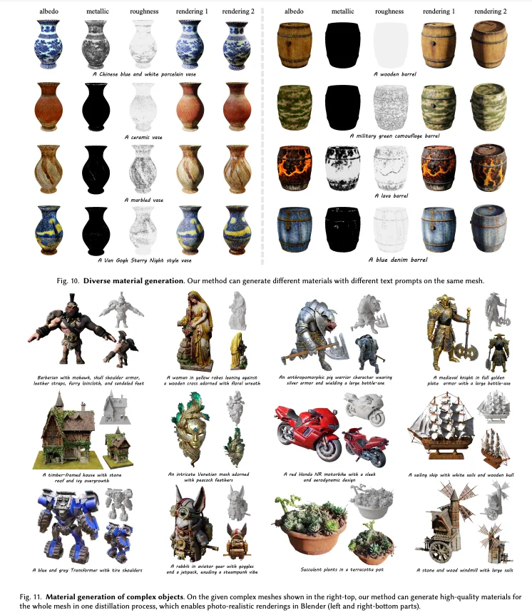
• A framework generating high-quality PBR materials—albedo, roughness, and metallic maps—for a specified mesh from text.

3. Method

3.1. Overview

A brief investigation of BRDF

The bidirectional reflectance distribution function (BRDF), alongside BTDF for transmission and BSDF for scattering, describes interactions between surfaces and light. BRDF describes how much light reflects in each direction after striking a surface. It is important for realistic PBR workflows.

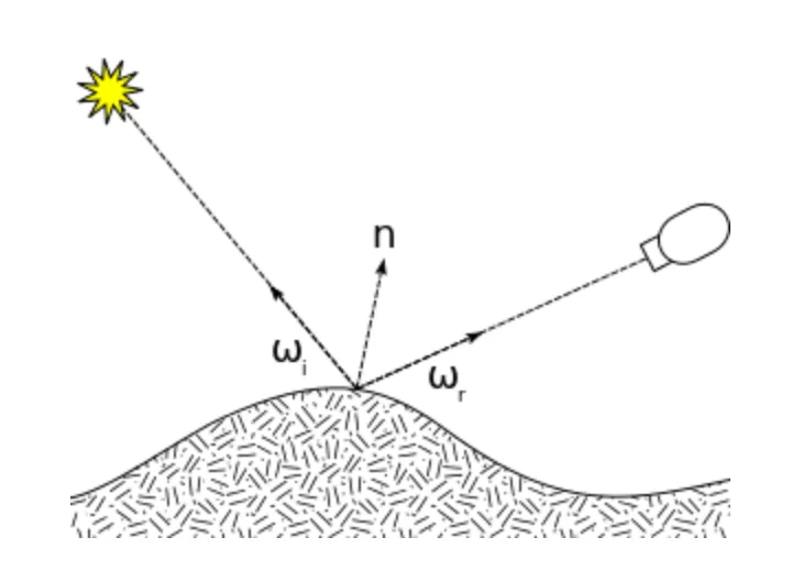
BRDF takes incoming and outgoing directions at a surface point and describes reflection in the outgoing direction. It is written as $f_r(\omega_i, \omega_r)$, with incoming-light direction $\omega_i$ and viewing direction $\omega_r$ as inputs.

 

A SVBRDF—spatially varying bidirectional reflectance distribution function—additionally takes surface position $\mathrm{x}$. $f_r(\omega_i, \omega_r, \mathrm{x})$

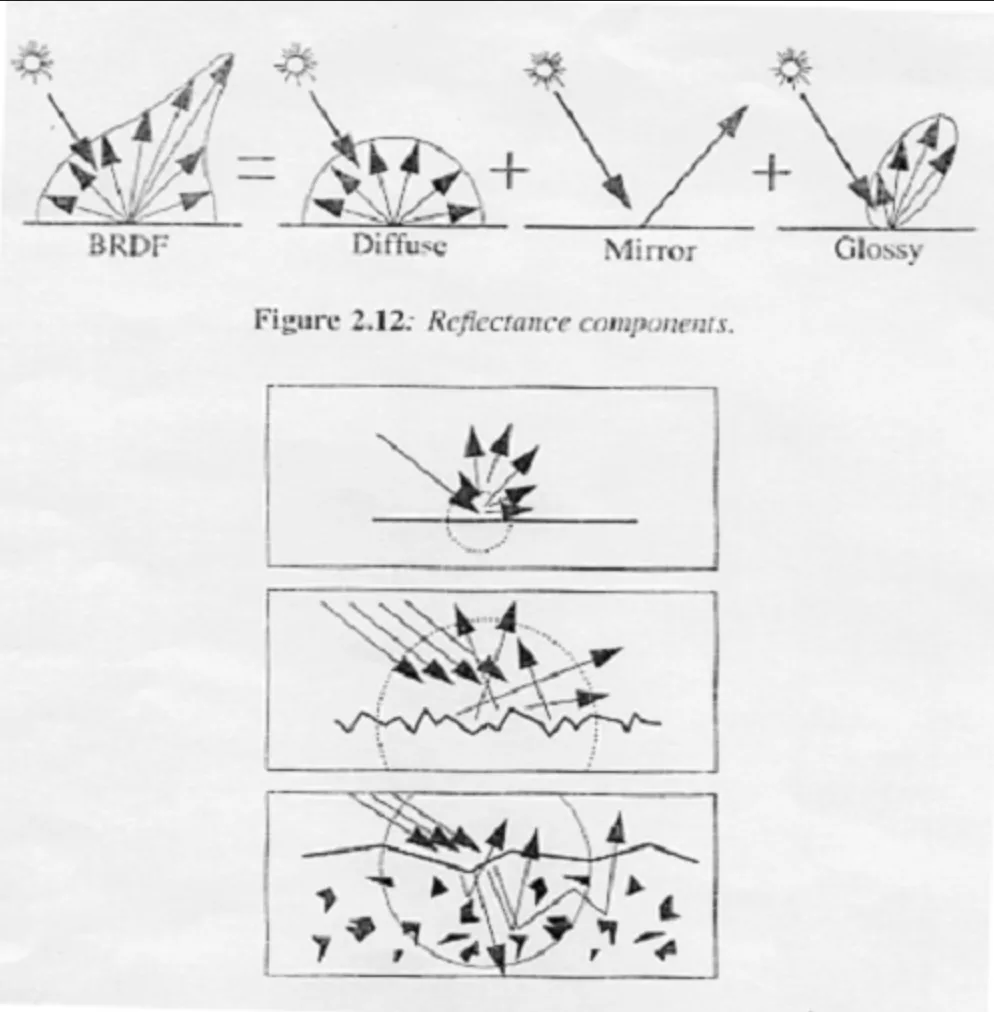
In short, BRDF and SVBRDF describe the interaction of an object with light, specifically its reflectance. Their differences are:

• BRDF: Assumes uniform reflective properties across the surface, the same at every point.

• SVBRDF: Allows reflective properties to differ at each surface point, representing complex real-world surfaces more accurately.

 

A simple illustration follows.

 

 

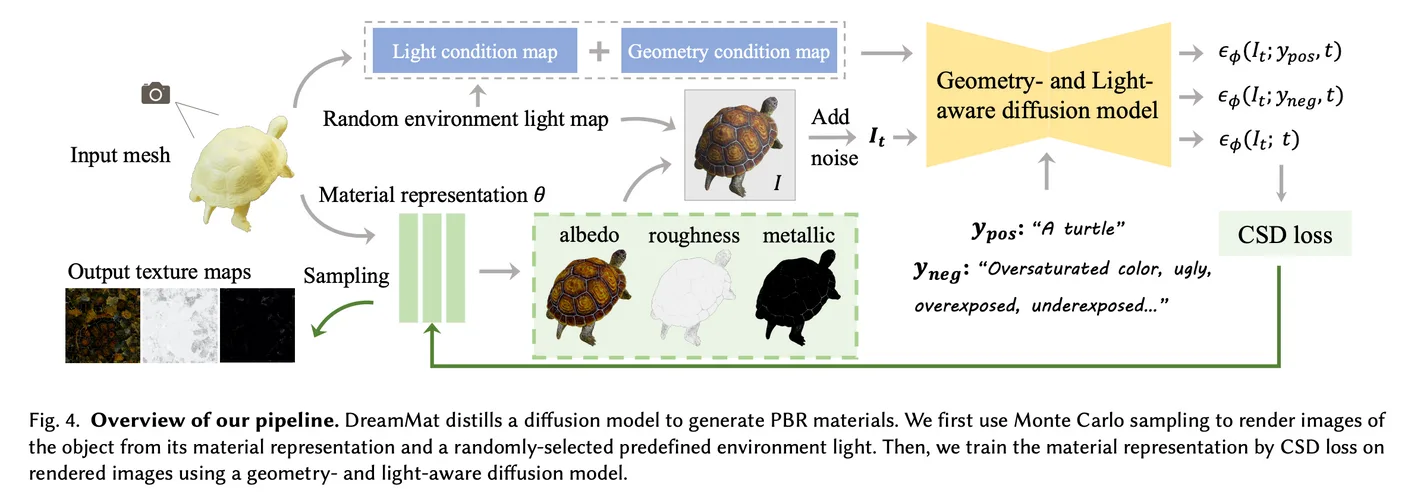
Given an untextured mesh and a prompt, DreamMat aims to generate SVBRDF materials. A hash-grid representation stores the material parameters and is used to render the mesh.

Noise is then added to the rendered image, which is passed through diffusion to obtain a distillation loss for training the hash-grid representation. Geometry- and light-aware diffusion avoids baked lighting and shadows. Generated materials can be exported as maps using supplied or extracted mesh UV coordinates.

3.2 Material Representation

This section introduces the material representation and rendering process. The paper uses Instant-NGP's hash-grid representation for a simplified Disney BRDF. At a point $p$, BRDF parameters including albedo $c$, roughness $\alpha$, and metallic value $m$ are calculated as follows.

Here, $\Gamma_\theta$ is the hash-grid representation with material parameters $\theta$. The goal is to learn $\theta$ so it can calculate BRDF parameters at every surface point $p$.

3.3 Distillation Loss for Material Generation

The material representation is randomly initialized and trained with an SDS loss. Noise $\epsilon_t$ is added to a rendered image $I$, producing $I_t = I + \epsilon_t$. Conditioned on prompt $y_{pos}$, the diffusion model produces $I^{\prime}_t$. The difference $\delta(I_t) = I^\prime_t - I$ between generated and rendered images forms distillation loss $\mathcal{L}_{Distill}$. Its gradient below trains $\theta$.

When diffusion denoises $I_t$ into $I^\prime_t$, $I^\prime_t$ should match the prompt better than $I$. Minimizing their difference $\delta(I_t) = I^\prime_t - I$ therefore aligns the rendering with the prompt. The equation gradually optimizes material parameters $\theta$ to achieve this. A rather obvious explanation...

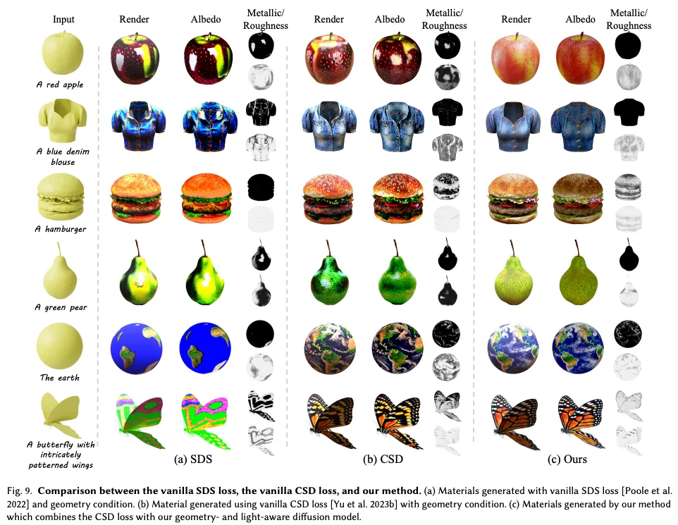
The authors adopt classifier score distillation, a variant of SDS that performs better in the figure above. The equation appears to add negative prompts such as 'oversaturated,' 'ugly,' 'underexposed,' and 'overexposed.' CSD seems to bring the CFG concept into SDS, enabling negative prompts; carefully chosen ones then improve results.

3.4 Geometry- and Light-aware Diffusion Model

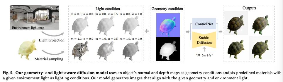
The authors fine-tune Stable Diffusion with ControlNet inputs for geometry and lighting. Geometry conditions are normals and depth. Lighting conditions use predefined materials with white albedo and several roughness/metallic combinations, rendered under different lights. These renderings feed the light ControlNet, trained using Objaverse. Since normal and depth ControlNets already exist, perhaps only the lighting component is newly trained? The result is generation consistent with geometry and lighting. Training the light ControlNet seems to be the main contribution.

3.5 Material Generation

The material-generation process first precomputes five random lighting conditions for each of 128 random viewpoints of the input mesh. At each distillation step, the current material representation is rendered under a random view and environment light. Diffusion then supplies a CSD loss to train its parameters. A material-smoothness loss additionally smooths roughness, metallic, and albedo values.

Finally, the learned representation $\Gamma_\theta$ is sampled into UV maps for use in an engine.

4. Experiment

4.1 Implementation Details

The geometry- and light-aware ControlNet trains on the Objaverse LVIS subset, using Stable Diffusion 2.1 and eight V100 GPUs.

5. Limitation and Conclusion

5.1 Limitation

• Metallic and roughness values can be inaccurate.

• It cannot represent transparency or strong reflections because the BRDF model cannot express those complex materials.

• It considers only direct light from the environment map, not indirect light reflected by the object itself. Highly reflective objects may therefore have inaccurate materials.

• Generation is slow, taking around twenty minutes.