TRELLIS: Structured 3D Latents for Scalable and Versatile 3D Generation

Paper: https://arxiv.org/abs/2412.01506 Project Page: https://trellis3d.github.io/ Github: https://github.com/microsoft/TRELLIS?tab=readme-ov-file

1. Introduction

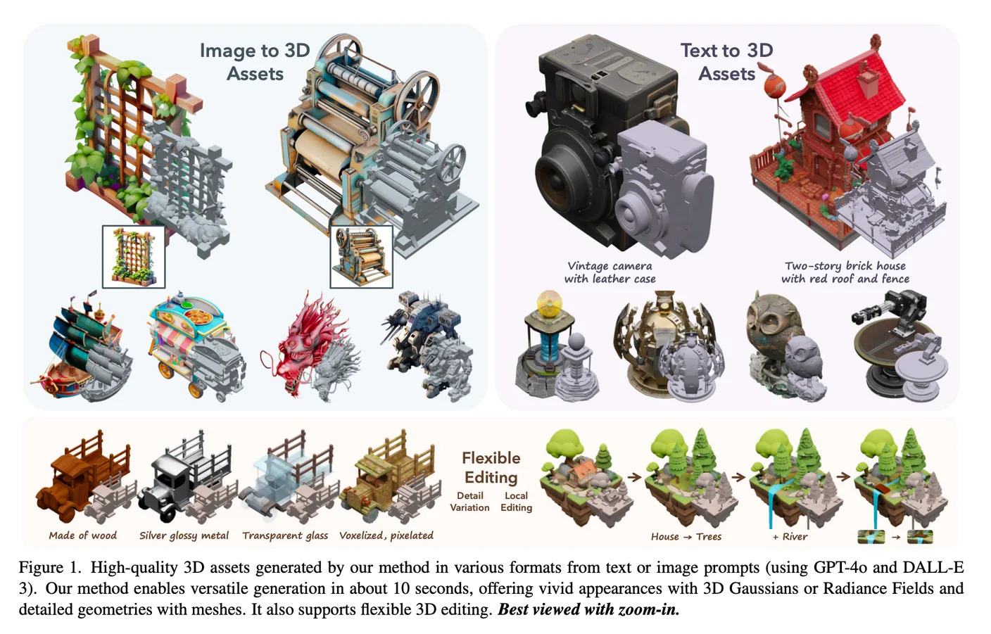
AI-generated 3D content has advanced considerably, but is not yet as ready for practical use as 2D image generation. Unlike 2D images, generally represented as pixel grids, 3D has many representations: meshes, point clouds, radiance fields, and 3D Gaussians. Mesh- and implicit-field-based generation struggles with detail, while 3DGS and NeRF methods struggle to extract convincing geometry. Each representation's structural properties also make a single architecture difficult. This contrasts with 2D models that learn in unified latent spaces using standardized approaches such as latent diffusion and flow. The paper therefore raises a fundamental problem of 3D representation.

Its solution is SLAT, a structured latent representation combining sparse structure with strong visual features and supporting decoding into radiance fields, 3D Gaussians, and meshes. It defines local latents for active voxels intersecting an object's surface, then combines them with detailed geometric and visual features extracted by DINOv2 from densely rendered multi-view images. In short, it first selects essential surface voxels, then attaches structural and visual details—textures, colors, and more—from multi-view images to create local latents. Decoders map SLAT into various high-quality 3D representations.

The paper also proposes TRELLIS, a large text- or image-conditioned 3D generative model based on SLAT. Its two-stage pipeline first generates sparse structure, then latent vectors for nonempty cells. It uses a rectified-flow transformer backbone, training models with up to two billion parameters on roughly 500,000 carefully collected 3D assets.

3. Method

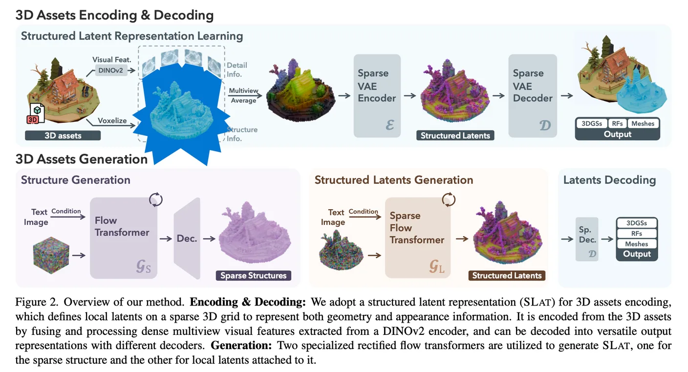
3.1. Structured Latent Representation

For a 3D asset $O$, geometry and appearance are encoded into a unified structured latent $z$, defined as local latents on a 3D grid.

$p_i$ indexes active voxels intersecting the surface of $O$, and $z_i$ is each voxel's associated local latent. N is the grid's spatial dimension; L is the total number of active voxels. Active voxels $p_i$ describe coarse structure, while latents $z_i$ describe appearance and shape detail. Together they cover the entire surface of $O$, capturing both overall shape and detail.

Because 3D data is sparse, active voxels are far fewer than all grid cells ($L << N^3$), enabling relatively high-resolution generation. The default N is 64, with an average L of 20,000.

3.2. Structured Latents Encoding and Decoding

Introducing the SLAT encoder and decoders for radiance fields, 3D Gaussians, and meshes.

3.2.1. Visual feature aggregation

First, asset $O$ is converted to voxelized features $f=\{(f_i, p_i)\}^L_{i=1}$. Here, $p_i$ denotes the active voxels defined in Equation 1, and $f_i$ is the visual feature containing detailed local structure and appearance.

To obtain each active voxel's $f_i$, the authors aggregate features from dense multi-view images of $O$. Cameras randomly sampled on a sphere render images, and DINOv2 extracts feature maps. Each voxel is projected to corresponding map locations; their average becomes $f^i$, as in Figure 2's upper left. The feature resolution matches structured latents $z$, at $64^3$. DINOv2's expressive features and the coarse voxel structure empirically suffice for accurate reconstruction.

3.2.2. Sparse VAE for structured latents

A transformer-based VAE encodes 3D assets using voxelized features $f$.

Encoder $\mathcal{E}$ maps $f$ to structured latent $z$, and decoder $\mathcal{D}$ maps $z$ to a specific representation. They train with reconstruction loss between the decoded and original assets, plus a KL penalty encouraging $z_i$ to follow a normal distribution.

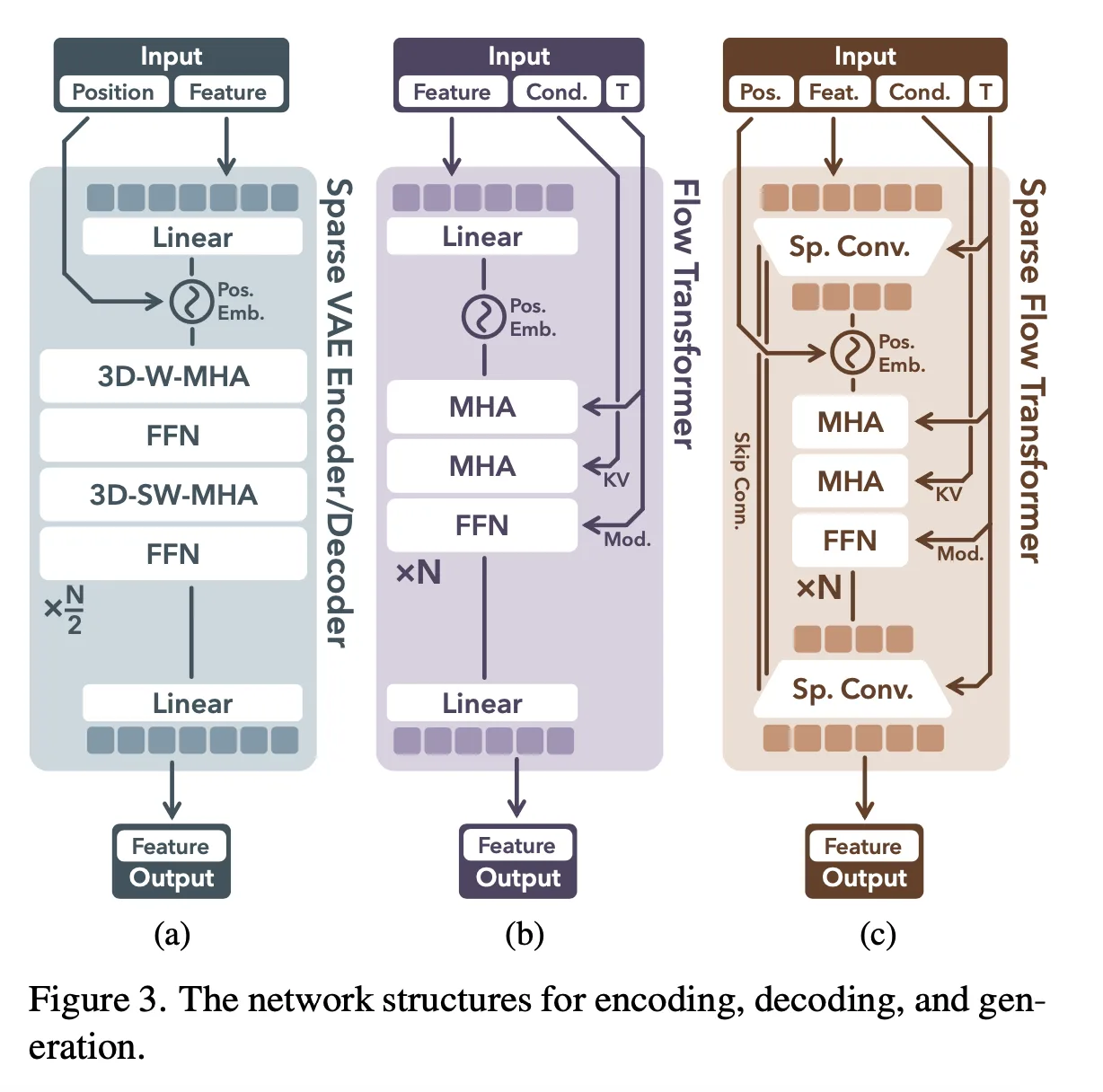
Encoder and decoder share the transformer architecture in Figure 3(a). Active-voxel features are serialized into variable-length token sequences of length L, with sinusoidal position encodings based on voxel locations. Transformer blocks then process them. Shifted-window attention in 3D strengthens local interactions and is more efficient than full attention.

3.2.3. Decoding into versatile formats

SLAT supports decoding into 3D Gaussians, radiance fields, and meshes, with decoders $\mathcal{D}_{GS}$, $\mathcal{D}_{RF}$, and $\mathcal{D}_{M}$. They share an architecture except for their output layers and train with representation-specific reconstruction losses.

(a) 3D Gaussians

Each $z_i$ decodes into K Gaussians with positional offsets $o$, colors $c$, scales $s$, opacities $\alpha$, and rotations $r$. Final positions $x$ stay near the active voxel to preserve the locality of $z_i$ ($x^k_i = p_i+tanh(o^k_i)$). Reconstruction compares rendered Gaussians with ground-truth images using $\mathcal{L}_1$, $D-SSIM$, and $LPIPS$.

(b) Radiance Fields

$v^x_i,v^y_i,v^z_i∈R^{16×8}$ and $v^c_i ∈ R^{16×4}$ are CP decompositions representing local radiance volumes at resolution $8^3$. Reconstruction loss resembles the Gaussian case.

(c) Meshes

$w^j_i \in \mathbb{R}^{45}$ contains FlexiCubes parameters, and $d^j_i \in \mathbb{R}^8$ gives signed distances at the eight voxel corners. Two convolutional upsampling blocks increase the output resolution to $256^3$. Meshes are extracted at the zero-level isosurface. Reconstruction uses $\mathcal{L}_1$ between rendered depth/normal maps and ground truth. The code appears to handle textures in the mesh decoder too; details from Appendix A.2 follow.

Mesh Decoder Detail

Two sparse convolutional upsamplers follow the transformer backbone, increasing spatial size from $64^3$ to $256^3$. Mesh extraction focuses on geometry, but also predicts color and normals. The final high-resolution active-voxel output is therefore:

Mesh extraction

Attach the sparse structure to a dense grid and extract a differentiable surface with FlexiCubes.

• For inactive voxels, set signed distance to 1.0 and other attributes to zero.

• Extract the mesh at the zero-level isosurface.

• Interpolate grid-vertex attributes, such as color and normals, at each extracted mesh vertex.

Render the mesh and its attributes using Nvdiffrast, producing:

• Foreground mask (M).

• Depth map (D).

• Normal map (N): Derived directly from mesh geometry.

• RGB image (C): The mesh's rendered color.

• Normal map (N): Generated from predicted normal values.

The training objective is as follows.

 

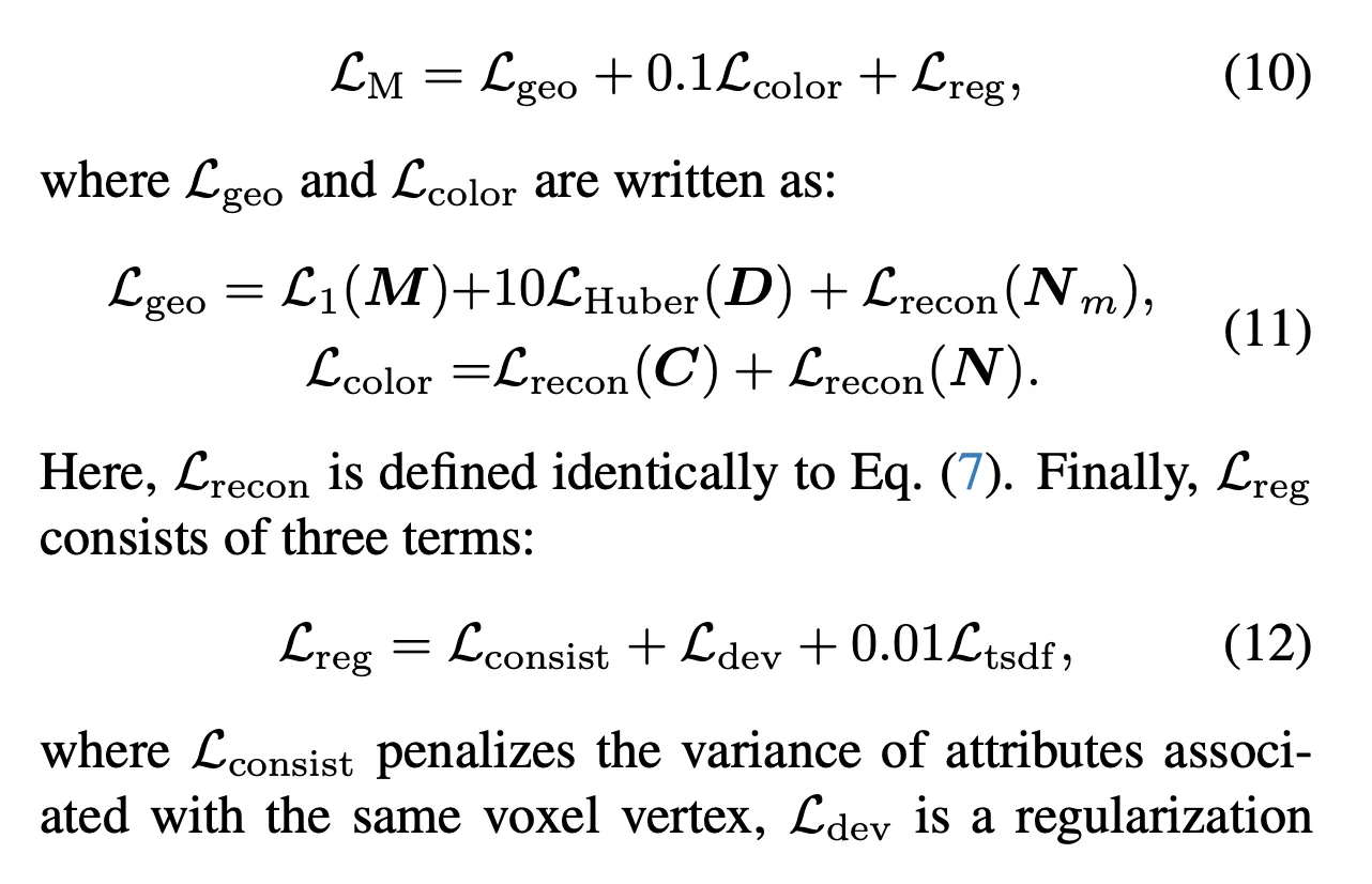
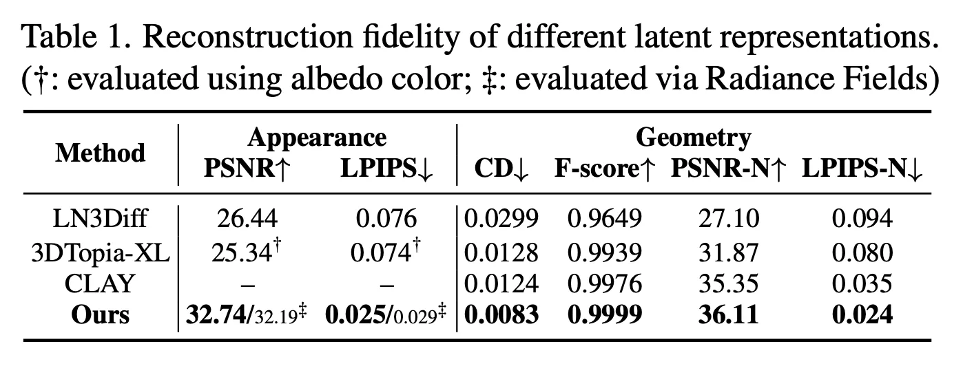
In practice, the encoder and Gaussian decoder train end to end. For other output formats, the trained encoder is frozen and a new decoder is trained. Gaussian-trained SLAT faithfully reconstructs assets in other formats, demonstrating extensibility; see Table 1. Appendix A.2 gives further implementation details.

3.3. Structured Latents Generation

SLAT generation uses two stages: sparse-structure generation, then generation of the associated local latents. Rectified flow models the latents.

3.3.1. Rectified flow models

Rectified flow uses a linear-interpolation forward process, $x(t) = (1-t)x_0 + t_\epsilon$, where $t$ is time, $x_0$ a data sample, and $\epsilon$ noise. It interpolates between data and noise. The reverse process uses a time-dependent vector field $v(x,t) = \nabla_tx$ to transport noisy samples to the data distribution. Refer to the flow literature for details.

3.3.2. Sparse structure generation

The first stage generates sparse structure $\{p_i\}^L_{i=1}$. To make this learnable by a neural network, active voxels become a dense binary grid $O \in \{0,1\}^{N \times N \times N}$, with 1 for active cells and 0 otherwise.

Directly generating dense grid $O$ is inefficient, so a simple 3D-convolutional VAE compresses $O$ into a lower-resolution feature grid $S \in \mathbb{R}^{D \times D \times D \times C_s}$. Because $O$ chiefly represents coarse shape, this compression loses little information and improves efficiency. It also converts discrete $O$ into continuous features suitable for rectified-flow training.

Transformer backbone $\mathcal{G}_S$ generates $S$, as in Figure 3(b). It receives a serialized noisy grid with position encodings. Adaptive layer normalization and gating integrate timestep information. CLIP supplies text conditions and DINOv2 supplies image conditions. Denoised feature grid $S$ decodes into discrete grid $O$, then active voxels $\{p_i\}^L_{i=1}$.

3.3.3. Structured latents generation

In the second stage, transformer $\mathcal{G}_L$ generates latents $\{z_i\}^L_{i=1}$ based on $\{p_i\}^L_{i=1}$, as in Figure 3(c). Unlike the sparse VAE encoder, it packs noisy latents into shorter sequences for efficiency, similarly to DiT. Using the first stage's sparse structure, it groups local latents and downsamples before serialization. Transformer blocks apply time-modulated processing; upsampling blocks and skip connections then transmit spatial information.

$\mathcal{G}_S$ and $\mathcal{G}_L$ train independently. Once trained, they generate SLAT $z=\{(z_i, p_i)\}^L_{i=1}$ sequentially, and decoders $\mathcal{D}_{GS}$, $\mathcal{D}_{RF}$, and $\mathcal{D}_{M}$ convert it into high-quality assets.

3.4. 3D Editing with Structured Latents

The model also supports flexible 3D editing with two simple tuning-free strategies.

3.4.1. Detail variation

Separating structure from latents allows detail changes without altering the overall coarse shape. Keep the structure fixed and run the second stage with a different prompt. This can also generate textures with fixed geometry.

3.4.2. Region-specific editing

SLAT's locality allows selected voxels and latents to change while other regions remain untouched. The authors adapt RePaint [55] to the two-stage pipeline. Given a bounding box, modified flow sampling generates new content inside it, conditioned on the unchanged region and the supplied text or image prompt.

4. Experiment

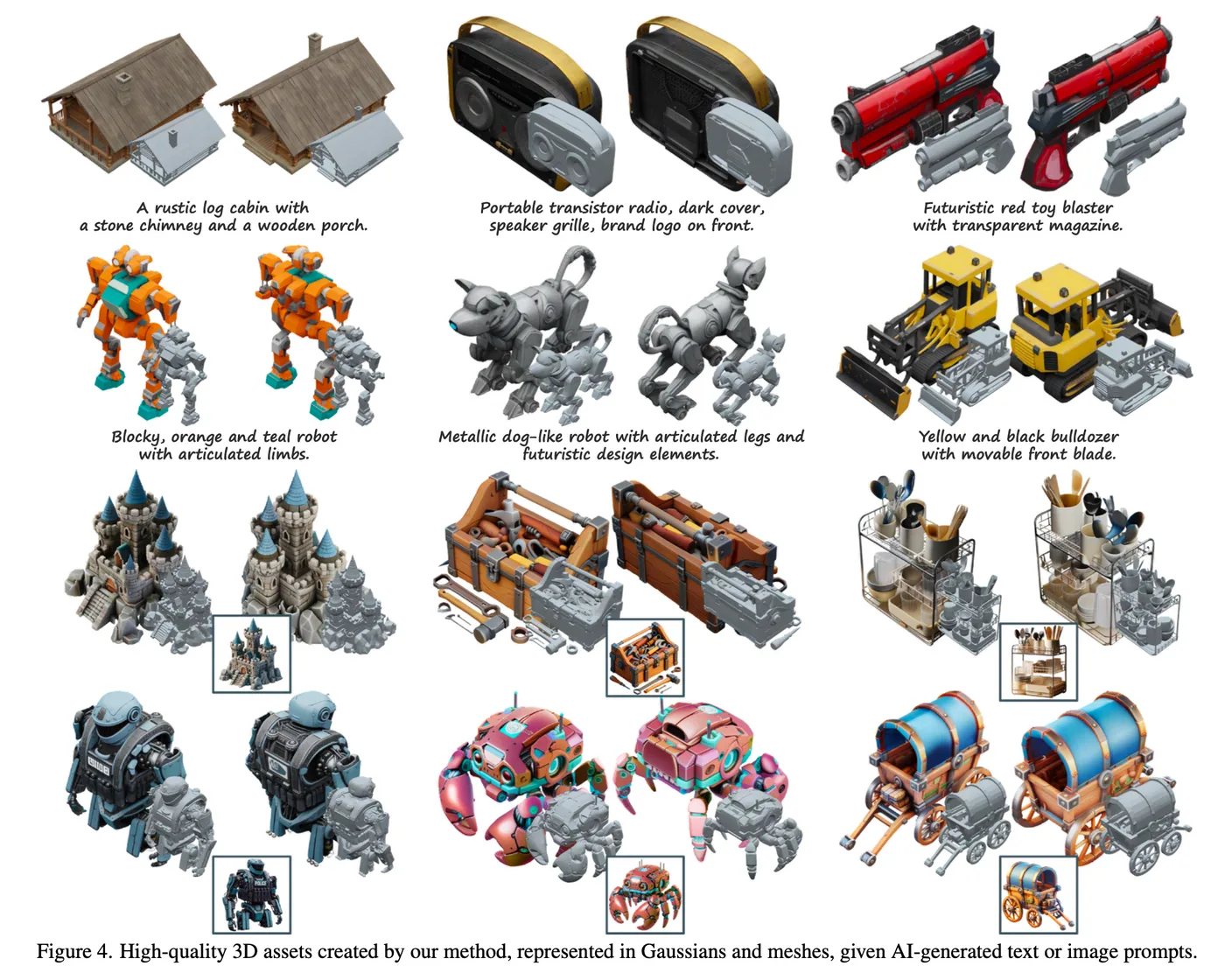
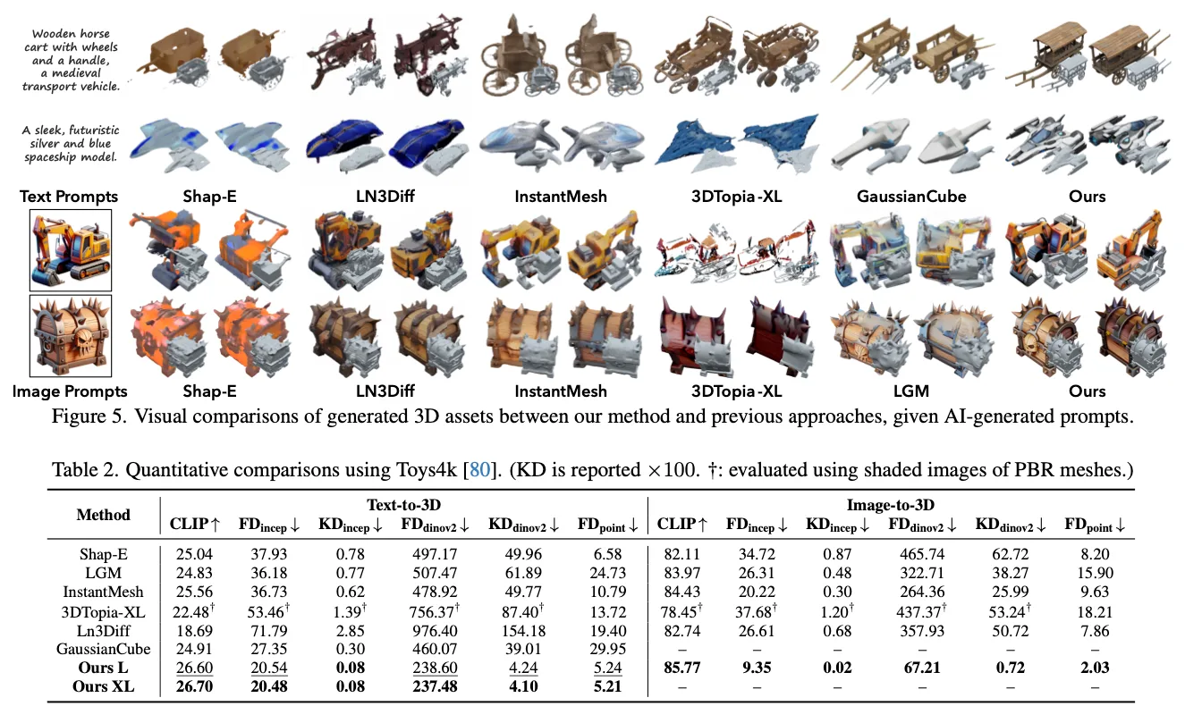
Implementation Details

TRELLIS trains on approximately 500,000 high-quality assets collected from Objaverse (XL), ABO, 3D-FUTURE, and HSSD. Each asset is rendered into 150 images and captioned with GPT-4o. Augmentation summarizes text into different lengths and renders image prompts with different fields of view.

Training uses AdamW, batch size 256, and 400,000 steps on 64 A100 GPUs with 40 GB memory. Model sizes are Basic, 342 million parameters; Large, 1.1 billion; and X-Large, 2 billion. Inference uses 50 sampling steps and CFG strength 3.

4.3. Ablation Study

4.3.1. Size of Structured Latents

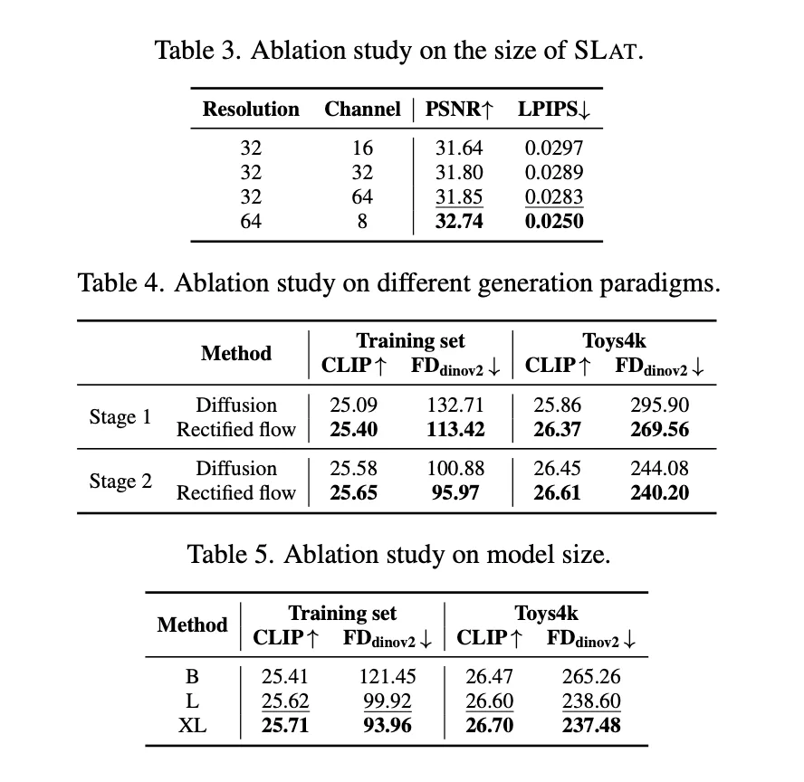
Sparse VAEs with different resolutions and channel counts determine SLAT size. Table 3 shows good performance even at $32^3$, with only marginal gains from more channels. Increasing resolution to $64^3$ improves performance substantially. Prioritizing quality over efficiency, the default SLAT configuration is $64^3$.

4.3.2. Rectified Flow v.s. Diffusion

Table 4 compares rectified flow with conventional diffusion by replacing the model in each pipeline stage. Replacing diffusion with rectified flow in either stage improves both generation quality and prompt alignment.

4.3.3. Model size

Table 5 evaluates different parameter counts. Larger models consistently improve generation performance on both the training distribution and the Toys4k dataset.

5. Limitation

Despite strong 3D generation performance, limitations remain.

First, the two-stage pipeline can be inefficient. Generating sparse structure and then its local latents may be less efficient than an end-to-end method producing a complete asset in one stage.

Second, lighting remains an issue. Image-conditioned generation does not separate lighting effects from assets, leaving reference-image shadows and highlights baked in. Potential improvements include stronger lighting augmentation for image prompts during training and adding PBR material prediction. These are directions for future research.