DDPM: Denoising Diffusion Probabilistic Models

DDPM: Denoising Diffusion Probabilistic Models

paper: https://arxiv.org/abs/2006.11239 github: https://github.com/lucidrains/denoising-diffusion-pytorch

1. Introduction

In short, DDPM gradually adds small Gaussian noise, with fixed time-dependent parameters, to an image until only normally distributed noise remains. The problem is how to reconstruct an image from that noise. Recovering an image from supplied noise becomes image generation.

The paper describes diffusion probabilistic models: parameterized Markov chains trained through variational inference to generate images after a finite number of steps. A Markov chain has the form $p(x|x)$, where the previous sample influences the current one. In one direction, small Gaussian noise is progressively added until the image is destroyed.

2. Background

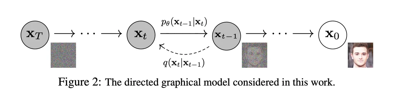
2-1. Forward Diffusion Process ($q$)

Let the original image be $x_0$ and the noising process $q$. Applying noise to $x_0$ to obtain $x_1$ is written $q(x_1|x_0)$, or generally at time t as $q(x_t|x_{t-1})$. This is the forward, or diffusion, process. It ends at $x_T$, pure noise following normal distribution $N(x_T;0,I)$. For equations, see the previous post.

2-2. Reverse Diffusion Process ($p$)

The reverse process gradually removes noise, opposite to $q$. Reversing time in $q(x_t|x_{t-1})$ gives $p(x_{t-1}|x_t)$. Note that$x_t$ all have the same resolution. For equations, see the previous post.

2-3. Objective Function ($L$)

The objective is to gradually remove noise from a given noisy sample, using $p$.

$x_t$ Given $x_{t-1}$ if we can predict this, we can $x_0$ also predict the following.

This operates through Gaussians parameterized by mean and variance. As a generative model, it maximizes generated-image log-likelihood, a measure of fit to the data distribution. The paper expresses this as minimizing negative log-likelihood.

Loss Function

The equation gives the variational bound on the right-hand side. Expanding it yields:

This is the resulting expression.

Notably, it directly compares the forward-process posterior and reverse process through KL divergence. Since the forward process is known and its posterior is closely related to the reverse process, the comparison is tractable.

A brief look at what posterior probability means

---

Link: https://hwiyong.tistory.com/27

1. Posterior

Posterior means probability after observation. Its counterpart is the prior; likelihood is another related quantity.

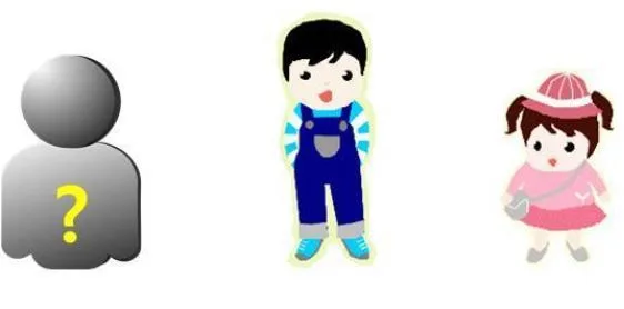
Suppose we observe a silhouette on a curtain. Consider two probabilities:

P(silhouette | Cheolsu) and P(Cheolsu | silhouette).

What we actually want is P(Cheolsu | silhouette).

This is the posterior, but we cannot usually calculate it directly. Variational inference and related methods

choose to approximate it rather than directly calculate the probability.

We use P(silhouette | Cheolsu), the likelihood, in that approximation.

• Inferring whether a silhouette belongs to Cheolsu may feel intuitive, but the reverse conditional can be less intuitive.

• P(silhouette | Cheolsu) considers the possible silhouettes Cheolsu could produce—animal-like, human-like, airplane-like, and so on.

• It gives the probability of observing the particular silhouette on the curtain among those possibilities.

Bayes' rule relates these quantities to the posterior.

$$P(철수|형상) = {P(형상|철수)P(철수) \over P(형상)}$$

The expression looks like conditional probability because it is the same concept.

We often rearrange it once more when approximating the quantity we want.

The denominator P(silhouette) is constant with respect to the alternatives in the numerator.

Ultimately,

$$P(철수|형상) \propto P(형상|철수)P(철수)$$

we approximate in the form below. Using more formal mathematical notation,

$$P(posterior) \propto likelihood \times P(prior)$$

we obtain this expression!

Known probabilities such as P(Cheolsu) and P(Yeonghui) are called priors.

Bayesian inference therefore obtains the posterior using likelihood and prior.

 

☞ Likelihood: p(z | x), the probability of observed data under a model.

☞ Prior probability: p(x), our probability for a system or model before observation. Population proportions such as p(man) and p(woman) are examples.

☞ Posterior probability: p(x | z), the probability of a model after observing an event.

---

Now consider the variational bound above.

3. Diffusion models and denoising autoencoders

3-1. Objective Function ($L$)

• The most important term is $L_{t-1}$. Starting from $x_0$ and expanding conditionally gives the tractable Gaussian forward posterior $q(x_{t-1}|x_t, x_0)$. Its KL divergence allows us to train the desired $p_\theta(x_{t-1}|x_t)$.

3-2. Forward Diffusion Process ($L_T$)

• The objective's first term

• Forward variances $\beta$ are fixed constants rather than learnable parameters, so $L_T$ can be ignored.

• Why?
• The forward process makes $x_T$ Gaussian, so tractable distribution$q(x_T|x_0)$ is very close to prior $p(x_T)$. Since forward variance is fixed, this approximate posterior contains no learnable parameters.
• Thus, this loss term is a constant near zero and is ignored during training.

3-3. Reverse Diffusion Process ($L_{1:T-1}$)

• The objective's second term

• First determine $q(x_{t−1}|x_t,x_0)$'s distribution, then obtain $\sum_\theta$ and $\mu_\theta$ to determine $p_\theta(x_{t−1}|x_t)$. We will examine them in order.

• (1) $q(x_{t-1}|x_t, x_0)$

As in the earlier diffusion overview, it is defined in the following form.

• $q(x_{t-1}|x_t, x_0) = N(x_{t-1}; \tilde{\mu}(x_t,x_0), \tilde{\beta}_t\mathrm{I})$
• $where, \tilde{\mu}_t(x_t,x_0) := {\sqrt{\bar{\alpha}_{t-1}}\beta_t\over1-\bar{\alpha_t}}x_0 \ + {\sqrt{\alpha_t}(1-\bar{\alpha}_{t-1})\over 1-\bar{\alpha}t}x_t, \ \tilde{\beta_t} := {(1-\bar{\alpha}_{t-1})\over 1-\bar{\alpha}_t}\beta_t$

• (2) $p_\theta(x_{t-1}|x_t)$

As in the earlier diffusion overview, it is defined in the following form.

• $p_\theta(x_{t-1}|x_t) = \mathcal{N}(x_{t-1}; \ \mu_\theta(x_t, t), \ \sum_\theta(x_t, t))$

• (3) $\sum_\theta(x_t, t)$

The standard deviation of $p$ is a constant matrix $\sigma_t^2 I$, so it need not be learned. Although $\sigma_t^2$ is more properly expressed as $\tilde{\beta_t}$, using $\beta$ is also acceptable.

• $\sum_\theta(x_t, t) = \sigma_t^2 I$

• (4) $\mu_\theta(x_t, t)$

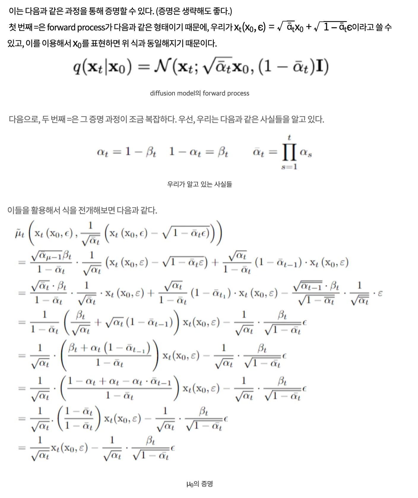
Finally, the mean $\mu_\theta(x_t, t)$ of $p$ is defined as follows.





Proof

 
 

• (5) Sampling

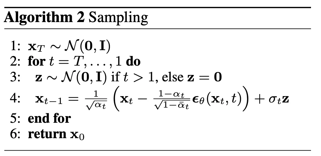
Once we obtain $\mu_\theta$, we can sample $x_{t-1}$ from $p_\theta(x_{t-1}|x_t)$ with the algorithm below.

• (6) $L_{t-1}$

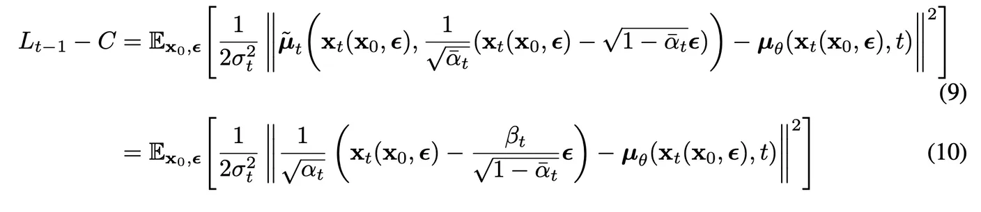
Combining $q$, $p_\theta$, and $\sum_\theta$ to calculate $D_{KL}$, the KL divergence, gives $L_{t-1}$ as follows.

The expectation changes from q to $x_0$ and $\epsilon$. This is natural because the forward Gaussian at any time can be reparameterized given the time and $x_0$.

• (7) $L_{simple}(\theta)$

Finally, rewrite the loss in terms of epsilon. This simplified objective improves training.

The simplified objective is effective because it trains the network at large t as well as very small t.

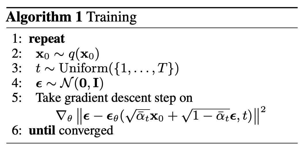
• (8) Training

DDPM training can therefore be summarized in the following short algorithm.

• (9) $L_0$

The final loss component $L_0$ is a simple KL divergence between two normal distributions and has the form below.

4. Experiments

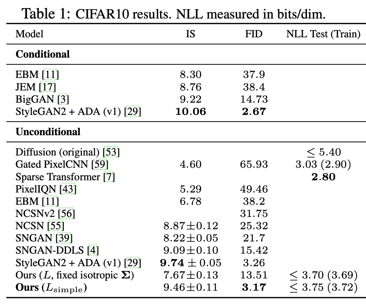
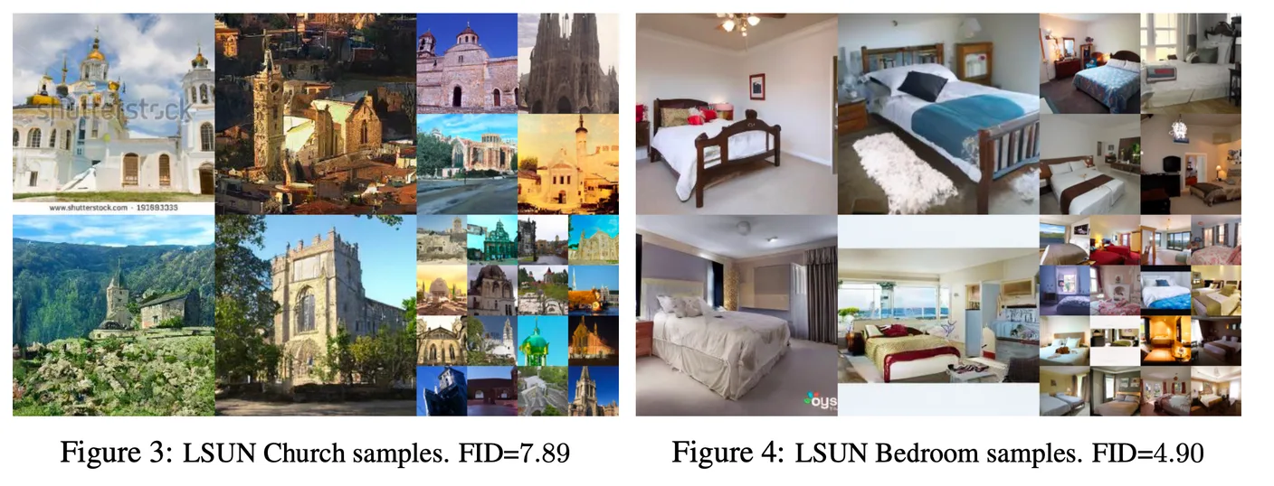
The central contribution is a convenient reparameterization of reverse-process $L_{t-1}$. Defining forward and reverse processes this way produces a generative model that synthesizes high-quality images.

References

1. Ho, J., Jain, A., & Abbeel, P. (2020). Denoising diffusion probabilistic models.  Advances in Neural Information Processing Systems, 33, 6840-6851.

2. https://lilianweng.github.io/posts/2021-07-11-diffusion-models/

3. https://deepseow.tistory.com/37

4. https://process-mining.tistory.com/188