Jan 27, 2021

(7) SARSA and Q-Learning

This is the seventh review post in my series on Reinforcement Learning with Python and Keras.

http://www.yes24.com/Product/Goods/44136413

Chapter 4. Reinforcement Learning Basics III: SARSA and Q-Learning SARSA Explaining the SARSA code SARSA's limitations Q-learning Explaining the Q-learning code Summary

Chapter 4. Reinforcement Learning Basics III: SARSA and Q-Learning

Policy and value iteration develop into SARSA. Beginning with 살사, we call these methods reinforcement learning. Let us see how iteration leads to SARSA and how agents learn with it.

SARSA

Policy iteration alternates policy evaluation with policy improvement. Evaluation finds the current policy's true value function through the Bellman expectation equation; improvement updates the policy using those values. This is GPI(Generalized Policy Iteration). In GPI, a single evaluation update is immediately followed by improvement, repeatedly.

GPI evaluates through the Bellman equation, while reinforcement learning uses Monte Carlo prediction or temporal-difference prediction. Greedy improvement in GPI obtains a policy for all states. Temporal-difference methods update only the current state's value at each timestep, so cannot improve every state simultaneously.

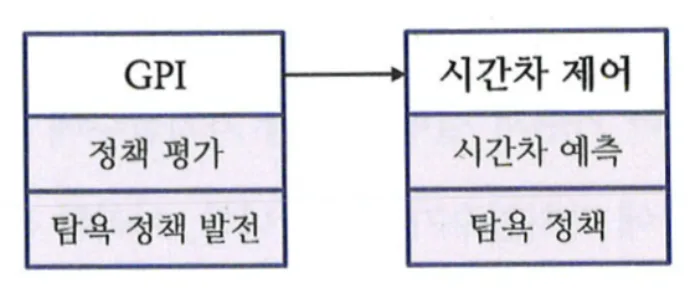
Temporal-difference methods therefore borrow from value iteration, which acts greedily on values without maintaining a separate policy. The agent uses 탐욕 정책, selecting the highest-value action in its current state. Combining temporal-difference prediction with a greedy policy gives 시간차 제어(Temporal-difference control). Their relationship is shown below.

GPI와 시간차 제어의 관계 — GPI and temporal-difference control

Using current-state Q-values rather than next-state values avoids needing the environment model. GPI needs transition probabilities $P_{ss'}^a$ to calculate $E_\pi [R_{t+1}+ \gamma v_\pi(S_{t+1})]$ —including the chance an action unexpectedly goes elsewhere. These belong to the environment and are hard to know in reality. Temporal-difference control selects actions through a Q-based greedy policy.

\pi (s) = argmax_{a \in A} \\\, Q(s,a)

Since action selection requires Q-values rather than state values, updates must target the Q-function. The 시간차 제어 equation therefore becomes:

Q(S_t, A_t) \leftarrow Q(S_t, A_t) + \alpha (R_{t+1} + \gamma Q(S_{t+1}, A_{t+1}) - Q(S_t, A_t))

Temporal-difference control needs samples to update Q-values. It uses $[S_t, A_t,R_{t+1}, S_{t+1}, A_{t+1}]$ . The interaction proceeds as follows.

In $S_t$ , the agent selects $A_t$ through its greedy policy.

The environment provides reward $R_{t+1}$ and next state $S_{t+1}$ .

In $S_{t+1}$ , the agent selects next action $A_{t+1}$ through its greedy policy.

The sample's form gives temporal-difference control the name 살사(SARSA). SARSA repeatedly collects samples using its current Q-function and policy, then updates the visited state–action values.

Early greedy behavior can lead to poor learning. To avoid converging to incorrect Q-values, the agent needs diverse experiences. A $\epsilon$ -greedy policy chooses a nongreedy action with probability $\epsilon$ .

Even after finding optimal values, a $\epsilon$ -greedy policy continues exploring with probability $\epsilon$ . We can therefore decrease $\epsilon$ as learning progresses.

\pi(s) = \begin{cases} \displaystyle a^* = argmax_{a \in A} \\\, Q(s,a), \\\,\\\,\\\, 1-\epsilon의\\\,확률로 \\\\ \displaystyle a \neq a^*, \\\,\\\,\\\,\\\,\\\, \epsilon의\\\,확률로 \end{cases}

SARSA can be summarized in two steps:

Collect sample $[S_t, A_t,R_{t+1}, S_{t+1}, A_{t+1}]$ with a $\epsilon$ -greedy policy.

Update Q-function $Q(S_t, A_t)$ using the sample and equation below.

Q(S_t, A_t) \leftarrow Q(S_t, A_t) + \alpha (R_{t+1} + \gamma Q(S_{t+1}, A_{t+1}) - Q(S_t, A_t))

Now let us examine the code.

Explaining the SARSA code


class SARSAgent:
  def __init__(self,actions):
    self.actions = actions # 에이전트가 할 수 있는 행동 [상,하,좌,우]
    self.step_size = 0.01      # α
    self.discount_factor = 0.9 # γ
    self.epsilon = 0.1         # ϵ
    self.q_table  = defaultdict(lambda: [0.0, 0.0, 0.0, 0.0])

Initialization sets the learning variables. To know which methods SARSAgent needs, consider how it interacts and learns:

Select an action in the current state through a $\epsilon$ -greedy policy.

Advance the environment one timestep with that action.

Receive reward and next state.

Select the next action with a $\epsilon$ -greedy policy.

Update Q-values using (s, a, r, s′, a′).

get_action receives a state and returns an action using a $\epsilon$ -greedy policy. It chooses greedily from q_table, or returns a random action according to the exploration probability.


# 입실론 탐욕 정책에 따라서 행동을 반환
def get_action(self, state):
    if np.random.rand() < self.epsilon:
        # 무작위 행동 반환
        action = np.random.choice(self.actions)
    else:
        # 큐함수에 따른 행동 반환
        state = str(state)
        q_list = self.q_table[state]
        action = arg_max(q_list)
    return action

After choosing actions in the current and next states, the agent learns from (s, a, r, s′, a′). The learn function implements the update below. It is very intuitive!

Q(S_t, A_t) \leftarrow Q(S_t, A_t) + \alpha (R_{t+1} + \gamma Q(S_{t+1}, A_{t+1}) - Q(S_t, A_t))


# <s, a, r, s', a'>의 샘플로부터 큐함수를 업데이트
def learn(self, state, action, reward, next_state, next_action):
    state, next_state = str(state), str(next_state)
    current_q = self.q_table[state][action]
    next_state_q = self.q_table[next_state][next_action]
    td = reward + self.discount_factor * next_state_q - current_q
    new_q = current_q + self.step_size * td
    self.q_table[state][action] = new_q

Using get_action and learn, the main loop interacts with the environment as follows.


# 행동을 위한 후 다음상태 보상 에피소드의 종료 여부를 받아옴
next_state, reward, done = env.step(action)
# 다음 상태에서의 다음 행동 선택
next_action = agent.get_action(next_state)
# <s,a,r,s',a'>로 큐함수를 업데이트
agent.learn(state, action, reward, next_state, next_action)

state = next_state
action = next_action

SARSA's limitations

SARSA uses a $\epsilon$ -greedy policy for sufficient exploration. Consider the situation below.

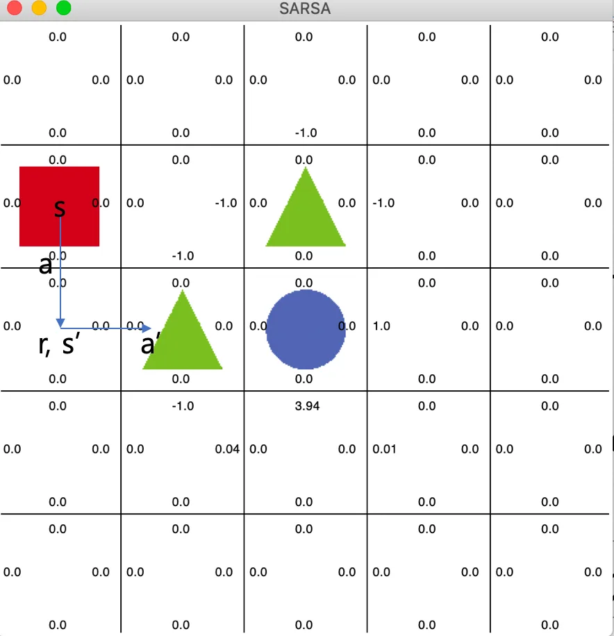
살사의 학습과정 중 한순간 — A moment during SARSA learning

Suppose an early agent takes $a$ in $s$ , then chooses next action $a’$ through exploration. It decreases $Q(s,a)$ , judging downward movement from $s$ undesirable. The agent may become trapped in a state. Learning from its own behavior is on-policy temporal-difference control. Off-policy temporal-difference control, 큐러닝, addresses this dilemma.

Q-learning

Off-policy means learning independently of the policy currently used to act: separate the behavior policy from the learning policy. Let us examine an example.

In state $s$ , the agent chooses $a$ using a $\epsilon$ -greedy policy, then receives reward $r$ and next state $s’$ , just as in SARSA. SARSA chooses another action with a $\epsilon$ -greedy policy and includes it in the sample. Q-learning, once it knows $s’$ , uses the largest Q-value in that state, $s’$ to update the current Q-value.

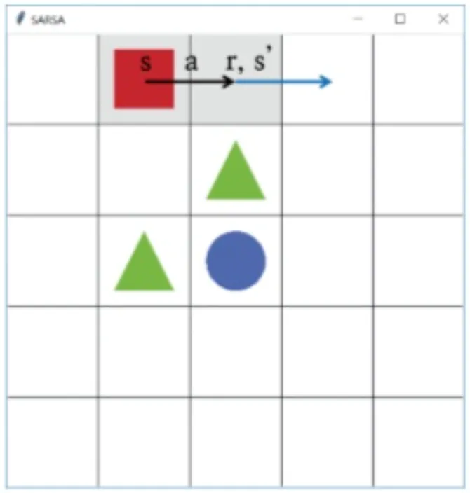
큐러닝의 학습과정 중 한순간 — A moment during Q-learning

Q-learning does not need to execute the next action in $s’$ ; it updates with the largest Q-value in $s’$ . This resembles the Bellman optimality equation.

Q(S_t, A_t) \leftarrow Q(S_t, A_t) + \alpha (R_{t+1} + \gamma max_{a'} Q(S_{t+1}, a') - Q(S_t, A_t))

The equation below is the Bellman optimality equation. Since reward $R_{t+1}$ is an actual observed value, removing the expectation gives the corresponding Q-learning target.

q^(s,a) = E[R_{t+1} + \gamma max_{a'} q^(S_{t+1},a') | S_t=s, A_t=a]

벨만 기대 방정식 –> 정책 이터레이션 –> 살사

벨만 최적 방정식 –> 가치 이터레이션 –> 큐러닝

Q-learning uses samples [s, a, r, s′]. Since acting and updating use different policies, it is 오프폴리시. Its simple Q-function formulation became a foundation for many later algorithms.

Explaining the Q-learning code

The difference from SARSA lies in learning from the samples.


# <s, a, r, s'> 샘플로부터 큐함수 업데이트
    def learn(self, state, action, reward, next_state):
        state, next_state = str(state), str(next_state)
        q_1 = self.q_table[state][action]
        # 벨만 최적 방정식을 사용한 큐함수의 업데이트
        q_2 = reward + self.discount_factor * max(self.q_table[next_state])
        self.q_table[state][action] += self.step_size * (q_2 - q_1)

learn implements the Q-learning update. Taking the maximum of self.q_table[next_state] makes it off-policy. No next-state action is needed.

The key difference is on-policy versus off-policy. In this gridworld example, SARSA's continued exploration can trap it in the upper-left corner. Q-learning learns independently of its behavior policy and can learn how to escape.

Summary

몬테카를로 예측: Replaces expectations with sampled averages.

V(s) \leftarrow V(s) + \alpha (G(s) - V(s))

시간차 예측: Unlike Monte Carlo prediction, updates at each timestep.

V(S_t) \leftarrow V(S_t) + \alpha (R_{t+1}+ \gamma V(S_{t+1}) - V(S_t))

살사(SARSA): Temporal-difference control using Q-values and samples (s, a, r, s′, a′).

Q(S_t, A_t) \leftarrow Q(S_t, A_t) + \alpha (R_{t+1} + \gamma Q(S_{t+1}, A_{t+1}) - Q(S_t, A_t))

큐러닝(Q-learning): Off-policy learning selects actions through a $\epsilon$ -greedy policy and updates Q-values using the Bellman optimality equation.

Q(S_t, A_t) \leftarrow Q(S_t, A_t) + \alpha (R_{t+1} + \gamma max_{a'} Q(S_{t+1}, a') - Q(S_t, A_t))