Jan 25, 2021

(6) Reinforcement Learning and Policy Evaluation

This is the sixth review post in my series on Reinforcement Learning with Python and Keras.

http://www.yes24.com/Product/Goods/44136413

Chapter 4. Reinforcement Learning Basics III: Reinforcement Learning and Policy Evaluation Human learning and reinforcement learning Prediction and control in reinforcement learning An example of Monte Carlo estimation Monte Carlo prediction Temporal-difference prediction

Chapter 4. Reinforcement Learning Basics III: Reinforcement Learning and Policy Evaluation

The difference between reinforcement learning and dynamic programming is that reinforcement learning learns an optimal policy through interaction without knowing the environment's model. The agent can learn the value function for a given policy through those interactions; this is called 예측. Continually improving the policy based on the value function to learn an optimal policy is called 제어.

Prediction includes 몬테카를로 예측 and 시간차 예측. Control includes 살사, a temporal-difference control method, and 큐러닝, an off-policy method that addresses SARSA's limitations.

Human learning and reinforcement learning

How can a reinforcement learning agent solve a sequential decision-making problem without a model? How does its learning work? 🧐

Consider dynamic programming. Its computational complexity grows exponentially as the number of states or dimensions increases, because it uses precise information about the environment to calculate values for all states together. It is like playing Go by considering every possible move. Do humans do that? No! Much of our learning comes simply from playing. Later, we review the game and consider where we went wrong and how to improve. This hints at how reinforcement learning works.

Reinforcement learning tries things, evaluates itself, updates itself based on that evaluation, and repeats the process many times.

Prediction and control in reinforcement learning

When solving a problem defined as an MDP, the key question is how to calculate the expectation in the Bellman expectation equation, $E_\pi$ . Repeating the calculations in policy iteration can produce the exact expectation, but relatively few problems allow this kind of dynamic programming.

People do not always base their judgments on exact information. Learning through reasonable inference, though less precise than iteration, is often more efficient in the real world. Reinforcement learning uses inference to 예측(prediction) the true value function. Improving a policy alongside prediction is called 제어(Control).

An example of Monte Carlo estimation

Normally, to calculate a circle's area, we find its equation ( $S = \pi r^2$ ) and use it. But what if we do not know the equation? How can we calculate the area?

We can use 몬테카를로 근사(Monte-Carlo Approximation). Monte Carlo means trying something at random, while estimation means using samples to infer an unknown true value. Estimating the original area by performing random trials is Monte Carlo estimation.

Imagine scattering points over a square sheet of paper (B) containing a circle (A). The proportion of points that fall inside A, together with the known $S(B)$ , lets us estimate $S(A)$ . More samples reduce the error; with infinitely many repetitions, the estimate approaches the true value.

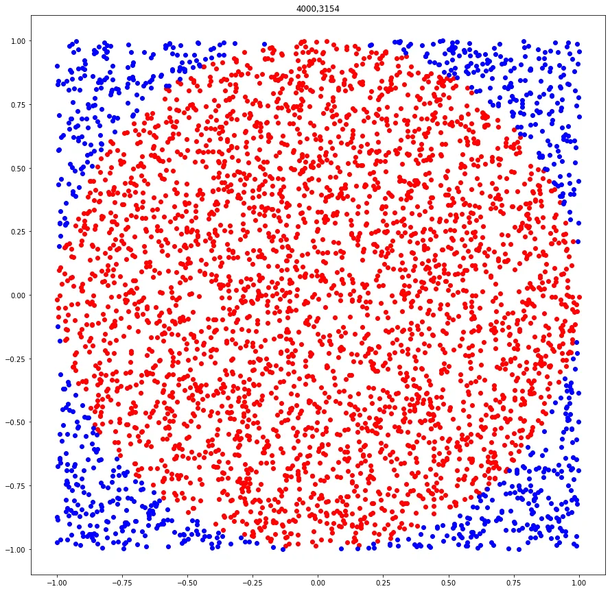
if \\\; n \to \infty, \\\, then \\\\ {1 \over n} \sum_{i=1}^n I(RedDot_i \in A) = {S(A) \over S(B)}

무수히 많은 점으로 원의 넓이를 추정 — Estimating a circle's area with many points

If we know the equation, we can find the area immediately. Why go to all this trouble? 😰 The advantage is that we can estimate the true value without knowing the equation. We can estimate the area of any shape, including the one below, even if we have no equation describing it. This ability to approach an answer through repetition without knowing the equation carries directly into reinforcement learning.

도형의 모양에 상관없이 몬테카를로 근사로 구할 수 있다 — Monte Carlo estimation works regardless of the shape.

Monte Carlo prediction

Instead of estimating a circle's area, let us estimate a value function. For the circle, each point was a sample, and placing points was sampling. For a value function, having the agent complete one episode in the environment is sampling. We estimate the true value function by averaging the samples. Using Monte Carlo estimation for this is called 몬테카를로 예측(Montecarlo Prediction).

Policy iteration explicitly calculates the expectation in the Bellman expectation equation. How can we instead predict a value function using sample averages, without calculating that expectation from the model?

Monte Carlo prediction does not calculate $E_\pi$ , which requires knowledge of the environment's model. Instead, it estimates $v_\pi (s)$ using the average return from multiple episodes, even without knowing the model.

v_\pi (s) \sim {1 \over N(s)}\sum_{i=1}^{N(s)}G_i(s)

One episode is not enough for a useful estimate, just as one point cannot estimate a circle's area. Monte Carlo prediction needs many returns for each state. Their average estimates that state's true value function.

Running many episodes under the current policy collects enough returns for all the states it can visit. We can therefore obtain a fairly accurate estimate of the value function.

Let us examine the averaging equation more closely, omitting the state notation for convenience. We denote the value estimate averaged over n returns by $V_{n+1}$ . The capital letter indicates that it contains estimation error. The update equation is derived as follows.

V_{n+1} = {1 \over n}\sum_{i=1}^n G_i = {1 \over n} \biggl( G_n + \sum_{i=1}^{n-1}G_i \biggl) \\\\ = {1 \over n} \biggl( G_n + (n-1)({1 \over n-1})\sum_{i=1}^{n-1}G_i \biggl) \\\\ = {1 \over n} ( G_n + (n-1)V_n) \\\\ = {1 \over n} ( G_n + nV_n - V_n) \\\\ = V_n + {1 \over n}(G_n - V_n) \\\\

We update a state's value function whenever the agent visits it through sampling, adding ${1 \over n}(G(s) - V(s))$ to the existing estimate $V(s)$ . Updating the average over time in this way is called 이동평균. The value-function update equation is shown below.

V(s) \leftarrow V(s) + {1 \over n}(G(s) - V(s))

In the equation, $G(s) - V(s)$ is the error, and ${1 \over n}$ is the 스텝사이즈(Step size) that determines how much of that error to use in the update. The step size is generally written as $\alpha$ , giving the general form below. A larger step size discounts older returns more rapidly, with exponential decay. (If the environment keeps changing, perhaps a fixed step size is preferable to averaging with 1/n?)

V(s) \leftarrow V(s) + \alpha (G(s) - V(s))

In Monte Carlo prediction, the agent uses this equation to update the value function for every state it experienced during the episode. As updates accumulate, the estimate converges toward the true value function for the current policy. Subsequent reinforcement learning methods use variations of this update equation, so understanding it precisely is important.

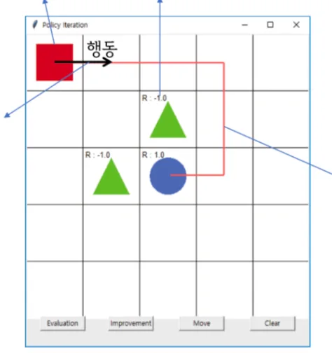
그리드월드에서 몬테카를로 예측 — Monte Carlo prediction in gridworld

One episode follows the red line. The agent makes no value updates until it reaches the terminal state, the blue circle. Then it updates the values of every state it visited. Once those updates are complete, it starts another episode from the beginning. Repeating this process is Monte Carlo prediction.

Temporal-difference prediction

A disadvantage of Monte Carlo prediction is that it does not update in real time. We must wait until an episode ends. It is also unsuitable for episodes that never end or last a very long time.

Unlike Monte Carlo prediction, 시간차 예측(Temporal-Difference Prediction) updates the value function at every time step. Just as people continually predict what happens next and learn immediately, it trains the agent in real time using the difference between its prediction and the observed target.

In Monte Carlo prediction, we could know $G_t$ only after an episode ended. Temporal-difference prediction instead uses the related definition below, expressing $G_t$ in terms of $R_{t+1} + \gamma v_\pi(s')$ . Rather than calculating an expectation as in dynamic programming, it samples $R_{t+1} + \gamma v_\pi(s')$ and uses that value to update the current estimate.

v_\pi (s) = E_\pi [R_{t+1}+ \gamma v_\pi (S_{t+1})|S_t = s]

Updates happen in real time. Unlike Monte Carlo prediction, it updates only one state's value function at a time. The agent retrieves the next state's estimate, $V(S_{t+1})$ , from its current list of values. It can then immediately calculate $R_{t+1} + \gamma v_\pi(s')$ , which becomes the update target for the value function of $S_t$ .

V(S_t) \leftarrow V(S_t) + \alpha (R_{t+1} + \gamma V(S_{t+1}) - V(S_t))

$R_{t+1} + \gamma V(S_{t+1}) - V(S_t)$ is called 시간차 에러(Temporal-Difference Error). Unlike the return, the temporal-difference update target is not an actual observed value. $V(S_{t+1})$ is merely the agent's current estimate; the agent predicts that it is the value of $S_{t+1}$ . Using another state's estimated value to estimate the current state's value is called 부트스트랩(Bootstrap). In other words, the value function is updated even though the target itself is not exact.

Temporal-difference prediction can update immediately without waiting for the episode to end. But will it still converge to the true value function, as Monte Carlo prediction does?

With enough sampled updates, it converges to the true value function. In many cases it approaches that value faster and more efficiently than Monte Carlo prediction. (The book does not explain this in detail... 😭) However, it has the disadvantage that prediction accuracy depends more strongly on the initial value estimates than in Monte Carlo prediction.

In the next post, we will examine the reinforcement learning algorithms 살사(SARSA) and 큐러닝(Q-learning)!