(4) Gridworld and Dynamic Programming

This is the fourth review post in my series on the book Reinforcement Learning with Python and Keras.

http://www.yes24.com/Product/Goods/44136413

Chapter 3. Reinforcement Learning Basics II: Gridworld and Dynamic Programming

So far, we have examined what a reinforcement learning problem is, how to define it mathematically, and how to formulate the equations for its optimal solution. Now it is time to solve a problem with a concrete example. 👉

다이내믹 프로그래밍(Dynamic Programming) is an efficient way to solve a large problem containing overlapping smaller problems by reusing the solution to one small problem in others.

Using dynamic programming:

• Solving the Bellman expectation equation → 정책 이터레이션

• Solving the Bellman optimality equation → 가치 이터레이션

In this chapter, we implement policy iteration and value iteration in code using a gridworld example.

Dynamic programming later becomes a foundation of reinforcement learning, so it is important to understand it properly!

Sequential decision-making problems

Reinforcement learning is one way to solve problems that require sequential decisions. Chapter 2 covered defining an MDP and formulating the Bellman equation. The steps for solving a sequential decision-making problem can be summarized as follows.

1. Convert the sequential decision-making problem into an MDP.

2. Repeatedly calculate the value function using the Bellman equation.

3. Obtain the optimal value function and optimal policy.

Since reinforcement learning also solves sequential decision-making problems, understanding it requires understanding the Bellman equation. But what does solving the Bellman equation mean? In mathematics, 'solving an equation' usually means finding values of the variables that satisfy it. The agent wants to find $v^*$ satisfying the equation below. Once those values are found, the equation has been solved and the agent knows 최적 가치함수.

Dynamic programming

The basic idea of dynamic programming is to break a large problem into overlapping smaller problems and solve them. Since the smaller problems are not independent, their solutions can be reused. This property ultimately reduces the amount of computation. (The book explains this at greater length; I have shortened it a little.)

Our goal is to find the true value function for each state.

That is, we want the true value of $v_\pi (s_1), v_\pi (s_2), v_\pi (s_3) …$. Breaking this large problem into smaller ones lets us solve it as shown below.

Each arrow represents one calculation, taking us from $iteration = k$ to $iteration=k+1$. We perform the calculation for all states, then update their value functions. In the next round, we repeat the same process using the updated values. This allows efficient updates based on information from the previous round.

A simple example on a grid: Gridworld

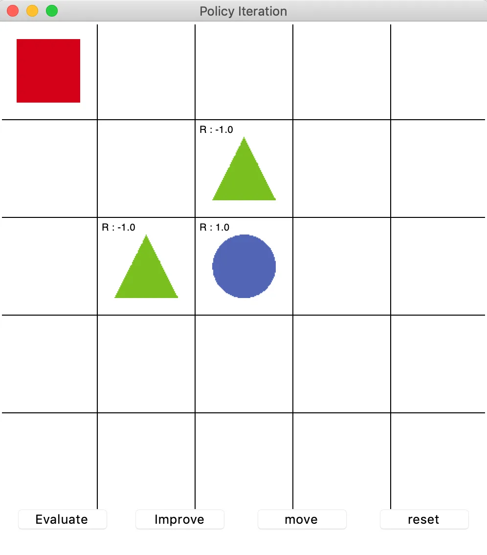
Here is the problem we will solve. The red square represents the agent, which must reach the blue circle. Light-green triangles stand in its way and give a reward of -1, so it must avoid them and reach the destination for a reward of +1. Our goal is to find an optimal policy for reaching the blue circle.

The flow of reinforcement learning algorithms

The diagram below shows the overall flow from an MDP to the basic reinforcement learning algorithms.

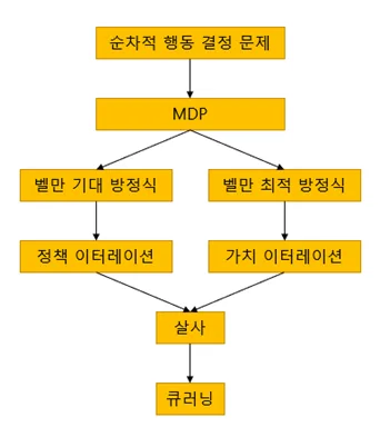
We have defined the sequential decision-making problem as an MDP. Its objective is to maximize the total reward the agent receives, which can be achieved by solving the Bellman equation. Dynamic programming can solve that equation, using 정책 이터레이션(policy iteration) or 가치 이터레이션(value iteration). These approaches later develop into 살사(SARSA), and SARSA leads to 큐러닝(Q-Learning).

Now let us train the agent using actual code!