Jan 24, 2021

(5) Policy Iteration and Value Iteration

This is the fifth review post in my series on Reinforcement Learning with Python and Keras.

http://www.yes24.com/Product/Goods/44136413

Chapter 3. Reinforcement Learning Basics II: Gridworld and Dynamic Programming Policy iteration Policy evaluation One policy-evaluation sweep proceeds as follows. Policy improvement Policy-iteration code policy_evaluation policy_improvement Value iteration Dynamic programming's limitations and reinforcement learning Model-free reinforcement learning Summary Chapter 3 in one sentence

Chapter 3. Reinforcement Learning Basics II: Gridworld and Dynamic Programming

Policy iteration

An MDP ultimately asks for the policy yielding the highest reward. Initially, we do not know it. We usually start with random actions and improve the policy.

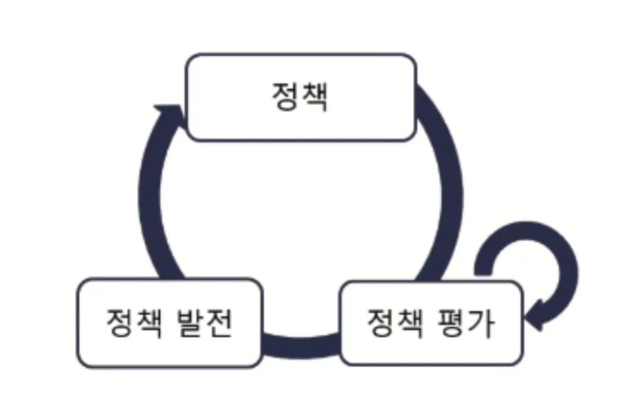
A random policy is not our desired optimum. We must evaluate and improve it. 정책평가(Policy Evaluation) assesses its quality, and 정책발전(Policy Improvement) improves it based on that assessment. Repeatedly doing this makes the policy converge to an optimal policy.

Imagining Professor Ahn's tough question 🤬: How can starting randomly possibly converge to an optimum? Explain in detail!

See the Pangyo Lab video around eighteen minutes: https://www.youtube.com/watch?v=rrTxOkbHj-M&t=19s

In short, even if neighboring values begin as nonsense, small pieces of information such as rewards gradually improve them toward the optimum. Like filtering water! I still find these updates remarkable.

정책평가와 정책발전 — Policy evaluation and improvement

Policy evaluation

The value function measures policy quality: the expected reward when following current policy. ⭐️ Since the agent seeks more reward, this information represents the policy's value.

v*\pi (s) = E[R*{t+1}+\gamma G\_{t+1}|S_t=s]

Policy iteration uses the Bellman expectation equation. The key is to calculate the next estimate from neighboring states' values and one timestep's reward. Since those values are not yet true values, one calculation is not exact. But repetition makes it converge to the true value.

The previous post converted this equation into a gridworld calculation. The equation below computes the (k+1)th estimate from the kth; we repeat it.

v_{k+1}(s) = \sum_{a \in A} \pi (a|s)(r_{(s,a)}+ \gamma v_k(s'))

One policy-evaluation sweep proceeds as follows.

From value matrix $k$ , retrieve $v_{k}(s’)$ stored at reachable next state $s’$ from current state $s$ , one of the purple cells.

Multiply $v_k(s')$ by discount factor $\gamma$ , then add reward $R_s^a$ for that action.

r_{(s,a)} + \gamma v_k(s')

Multiply the result by the policy's probability of taking the action.

\pi (a|s)(r_{(s,a)} + \gamma v_k(s'))

Repeat for every available action and sum the values.

v_{k+1}(s) = \sum_{a \in A} \pi (a|s)(r_{(s,a)}+ \gamma v_k(s'))

Store that sum at state $s$ in value matrix $K+1$ .

Repeat steps 1–5 for all $s \in S$ .

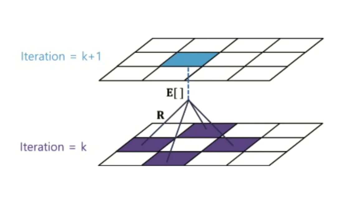
This completes one evaluation sweep, but one is not enough. Starting from v_1 and repeating indefinitely approaches the true $v_\pi$ .

Policy improvement

Evaluation alone is pointless if the policy never improves. There is no single mandatory improvement method, but the book uses the widely known 탐욕 정책 발전(Greedy Policy Improvement).

Compare the available actions' Q-values $q_\pi (s,a)$ in state $s$ and choose the largest. This is greedy policy improvement, named for pursuing the largest immediately apparent benefit.

The updated policy is below. Unlike max, its output is an action.

\pi'(s) = argmax_{a \in A} \\\; q_\pi (s,a)

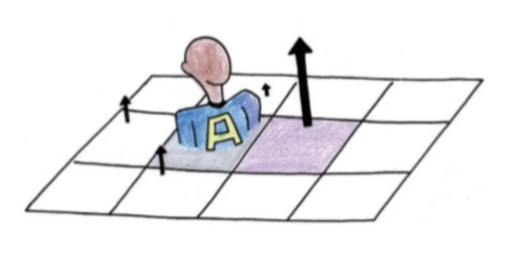
After greedy improvement, the updated policy's value is always greater than or equal to the previous value. Dynamic programming uses this to converge to a maximum-value optimal policy.

Policy-iteration code

Considering the agent's responsibilities, the code's overall flow is:


class PolicyIteration:
  def __init__(self, env):
    # 환경에 대한 객체
    self.env = env

  # 정책 평가
  def policy_evaluation(self):
    pass

  # 정책 발전
  def policy_improvement(self):
    pass

  # 특정 상태에서 정책에 따른 행동
  def get_action(self, state):
    return action

if __name__ == "__main__":
  env = Env()
  policy_iteration = PolicyIteration(env)
  grid_world = GraphicDisplay(policy_iteration)
  grid_world.mainloop()

The agent knows the following environment information:

env.width, env.height: Gridworld width and height.

env.state_after_aciton(state, action): The next state after a given action in a given state.

env.get_all_states(): All existing states.

env.get_reward(state, action): The reward for a particular state.

env.possible_actions: Up, down, left, and right.

Policy iteration comprises evaluation and improvement, so define a function for each.

policy_evaluation

Evaluation updates every state's value. After calculating the Bellman expectation equation for all states, policy_evaluation replaces value_table with next_value_table.

v_{k+1}(s) = \sum_{a \in A} \pi (a|s)(r_{(s,a)}+ \gamma v_k(s'))

This is the equation used for evaluation. Transition probability is set to 1, so choosing left leads to the state on the left.


# 벨만 기대 방정식을 통해 다음 가치함수를 계산하는 정책 평가
def policy_evaluation(self):
    # 다음 가치함수 초기화
    next_value_table = [[0.00] * self.env.width
                        for _ in range(self.env.height)]

    # 모든 상태에 대해서 벨만 기대방정식을 계산
    for state in self.env.get_all_states():
        value = 0.0
        # 마침 상태의 가치 함수 = 0
        if state == [2, 2]:
            next_value_table[state[0]][state[1]] = value
            continue

        # 벨만 기대 방정식
        for action in self.env.possible_actions:
            next_state = self.env.state_after_action(state, action)
            reward = self.env.get_reward(state, action)
            next_value = self.get_value(next_state)
            value += (self.get_policy(state)[action] *
                      (reward + self.discount_factor * next_value))

        next_value_table[state[0]][state[1]] = value

    self.value_table = next_value_table

$\sum_{a \in A}$ : for action in self.env.possible_actions:

$\pi (a|s)$ : self.get_policy(state)[action]

$r(s,a)$ : reward = self.env.get_reward(state, action)

$\gamma$ : self.discount_factor (0.9)

$s’$ : next_state = self.env.state_after_action(state, action)

$v_k(s')$ : self.get_value(next_state)

$v_{k+1}(s)$ : next_value_table[state[0]][state[1]]

get_policy retrieves action probabilities for each state. Add the action's reward to the discounted next-state value. Weighting and summing over all actions computes the expectation.

policy_improvement

Evaluation produces a new value function. The agent then improves its policy greedily using these values.


# 현재 가치 함수에 대해서 탐욕 정책 발전
def policy_improvement(self):
    next_policy = self.policy_table
    for state in self.env.get_all_states():
        if state == [2, 2]:
            continue

        value_list = []
        # 반환할 정책 초기화
        result = [0.0, 0.0, 0.0, 0.0]

        # 모든 행동에 대해서 [보상 + (할인율 * 다음 상태 가치함수)] 계산
        for index, action in enumerate(self.env.possible_actions):
            next_state = self.env.state_after_action(state, action)
            reward = self.env.get_reward(state, action)
            next_value = self.get_value(next_state)
            value = reward + self.discount_factor * next_value
            value_list.append(value)

        # 받을 보상이 최대인 행동들에 대해 탐욕 정책 발전
        max_idx_list = np.argwhere(value_list == np.amax(value_list))
        max_idx_list = max_idx_list.flatten().tolist()
        prob = 1 / len(max_idx_list)

        for idx in max_idx_list:
            result[idx] = prob

        next_policy[state[0]][state[1]] = result

    self.policy_table = next_policy

Greedy improvement chooses the highest-value action. If several actions tie, as in this example, the new policy selects them with equal probability.

Calculate $r_{(s,a)}+\gamma v_k(s')$ for each available action.

Store the calculated values in value_list.

Use max to find its largest value.

Use argwhere to obtain every maximizing index and store them in max_idx_list.

Calculate equal probabilities from the length of max_idx_list and store them in result.

policy_table now contains the updated action probabilities for every state.

In policy iteration, an agent repeatedly evaluates and improves its policy to find an optimal one.

정책 이터레이션으로 구한 최적 정책 — The optimal policy from policy iteration

Value iteration

The important difference is that policy iteration separates evaluation and improvement, whereas value iteration does not.

Value iteration treats its current estimates as estimates of optimal-policy values, so no separate improvement function is needed. get_action, returning optimal actions, displays the implied policy.

The overall code flow is:


class ValueIteration:
  def __init__(self, env):
    # 환경 객체 생성
    self.env = env

  # 벨만 최적 방정식을 통해 다음 가치함수 계산
  def value_iteration(self):
    return

  # 현재 가치함수로부터 행동을 반환
  def get_action(self, state):
    return

  def get_value(self, state):
    return

if __name__ == "__main__":
  env = Env()
  value_iteration = ValueIteration(env)
  grid_world = GraphicDisplay(value_iteration)
  gird_world.mainloop()

Policy iteration computes values through policy_evaluation and the expectation equation. Value iteration uses value_iteration instead.


# 벨만 최적 방정식을 통해 다음 가치 함수 계산
def value_iteration(self):
    # 다음 가치함수 초기화
    next_value_table = [[0.0] * self.env.width
                        for _ in range(self.env.height)]

    # 모든 상태에 대해서 벨만 최적방정식을 계산
    for state in self.env.get_all_states():
        # 마침 상태의 가치 함수 = 0
        if state == [2, 2]:
            next_value_table[state[0]][state[1]] = 0.0
            continue

        # 벨만 최적 방정식
        value_list = []
        for action in self.env.possible_actions:
            next_state = self.env.state_after_action(state, action)
            reward = self.env.get_reward(state, action)
            next_value = self.get_value(next_state)
            value_list.append((reward + self.discount_factor * next_value))

        # 최댓값을 다음 가치 함수로 대입
        next_value_table[state[0]][state[1]] = max(value_list)

    self.value_table = next_value_table

v_{k+1}(s) = max_{a \in A}(r_{s,a} + \gamma v_k(s'))

Calculate the Bellman optimality expression and store results in value_list.

Store the maximum as the new state value.


# 현재 가치 함수로부터 행동을 반환
def get_action(self, state):
    if state == [2, 2]:
        return []

    # 모든 행동에 대해 큐함수 (보상 + (감가율 * 다음 상태 가치함수))를 계산
    value_list = []
    for action in self.env.possible_actions:
        next_state = self.env.state_after_action(state, action)
        reward = self.env.get_reward(state, action)
        next_value = self.get_value(next_state)
        value = (reward + self.discount_factor * next_value)
        value_list.append(value)

    # 최대 큐 함수를 가진 행동(복수일 경우 여러 개)을 반환
    max_idx_list = np.argwhere(value_list == np.amax(value_list))
    action_list = max_idx_list.flatten().tolist()
    return action_list

Calculate Q-values for all actions.

Retrieve the index of every highest-value action.

Store those actions in action_list.

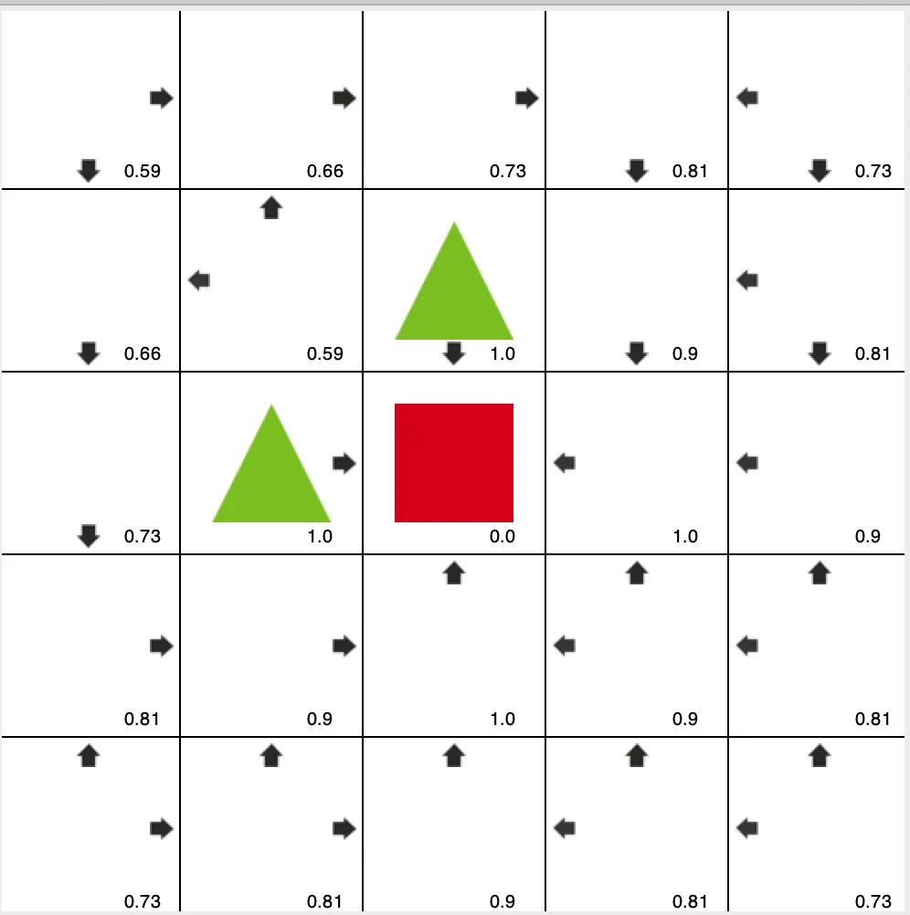
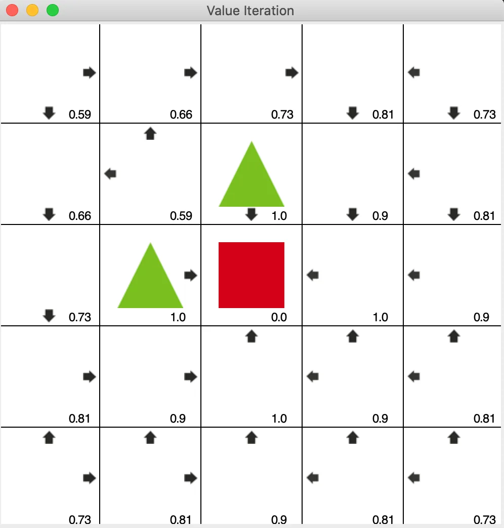
In this example, values nearly converge after around six Calculate operations. Displaying the policy from those values gives the figure below.

가치 이터레이션으로 구한 최적 정책 — The optimal policy from value iteration

Dynamic programming's limitations and reinforcement learning

We have examined Bellman-based policy and value iteration. But dynamic programming accelerates calculation rather than learning. What are its limitations?

1. Computational complexity: Large problems become hard to calculate; 계산복잡도 scales with the cube of the state count. 2. The curse of dimensionality: Gridworld states have two dimensions; increasing dimensions grows the state count exponentially. 3. Complete environment information: Exact rewards and transition probabilities are required, but usually unavailable.

These limitations are severe in real-world environments. To overcome them, methods learn from experience through interaction without knowing the environment. This is 강화학습.

Model-free reinforcement learning

In an MDP, the environment model consists of transition probabilities and rewards.

Model = P_{ss'}^a, \\\; r(s,a)

Here, a mathematical model is an equation describing a system's outputs for its inputs. Expressing that relationship mathematically is called 모델링(Modeling).

Such equations are never perfectly exact. A model may predict B from input A while reality differs. Greater accuracy increases complexity; exactly modeling natural phenomena such as air and wind is almost impossible. Human-made games obey defined rules, so we can regard them as having no modeling error. Outside games, though... 🤔

When the exact model is unknown, there are two approaches:

Model as accurately as possible, then experimentally adjust for modeling error.

Learn input–output relationships through interaction without a model.

The first is a traditional non-learning approach that provides system-stability guarantees, but encounters limits as complexity increases.

The second involves learning. It cannot guarantee identical behavior in every situation, but avoiding a model is advantageous for complex problems. This is 강화학습, the book's subject.

Summary

정책 이터레이션: Evaluate with the Bellman expectation equation and improve greedily.

가치 이터레이션: Assume an optimal policy and use the Bellman optimality equation; choose actions through Q-values without explicitly maintaining a policy.

다이내믹 프로그래밍의 한계: Computational complexity, dimensionality, and the need for complete environment knowledge.

Chapter 3 in one sentence

Writing briefly and clearly is actually harder...