(2) The Markov Decision Process

This is the second review post in my series on Reinforcement Learning with Python and Keras.

http://www.yes24.com/Product/Goods/44136413

Chapter 2. Reinforcement Learning Basics I: The Markov Decision Process

MDP

As we saw earlier, MDP mathematically represents a problem requiring sequential decisions.

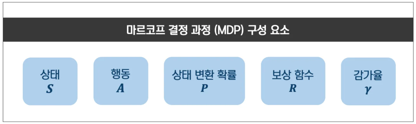
If we define the problem incorrectly, the agent may not learn at all. Problem definition is therefore one of the most important stages of learning. We must give the agent appropriate information—neither too much nor too little. To understand MDP, we will examine an example called 그리드 월드(Grid World). A gridworld is an environment arranged as a grid, used in various example problems. Let us examine each component of an MDP.

State

$S$ is the set of states observable by the agent. 'State' can sound vague; an observation of one's situation is the clearest description. For a real-world agent such as a robot, it might consist of sensor readings. For an agent learning a game, as in this book, we must define the states ourselves. It helps to ask: 'Does the state I defined provide enough information for the agent to learn?'

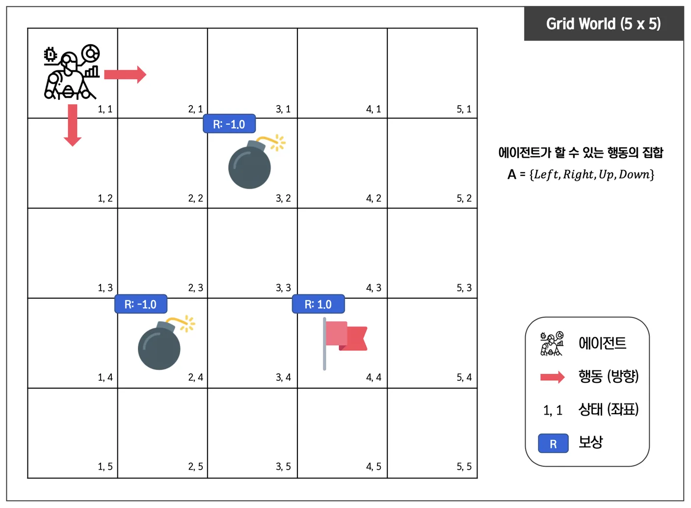
In the 5×5 gridworld shown above, each location, or coordinate, on the grid is a state. There are 25 states in total, corresponding to all grid positions. Each is an (x, y) coordinate, with the horizontal axis as x and the vertical axis as y. We can write this as follows.

Over time, the agent explores states in this set of 25. We denote time by t and the state at time t by $S_t$. If that state is (1, 3), we write $S_t=(1,3)$.

In MDP, the state changes probabilistically over time. At t = 1, it might be $S_t=(1,3)$ or $S_t=(4,2)$. The state occupied at time t is therefore a random variable. Rolling a die, for example, is a random experiment, and the resulting number is a variable with a probability of occurring. Such a variable is a random variable. We usually express 'the state at time t, $S_t$, is the particular state $s$' as $S_t=s$.

The state at an arbitrary time t → $S_t$

$S_t$ is a particular state $s$ → $S_t=s$

Action

The set of possible actions in state $S_t$ is $A$. Usually, the available actions are the same in all states, so they can be represented by a single set $A$. The action a at time t is written as $A_t=a$. Since the agent's action at time t is not predetermined, we use the capitalized $A_t$: it is a random variable.

In gridworld, the set of available actions is as follows.

If St = (3, 1) and At = right, then St+1 = (4, 1). However, an unexpected factor such as wind might prevent the agent from reaching (4, 1). What determines where it moves, including such factors, is called 상태 변환 확률. We will examine this in more detail shortly.

Reward function

Reward is information provided by the environment and the agent's learning signal. When St = s and At = a at time t, the reward function is defined as follows.

The reward function is the expected reward $E$ for taking action $A_t=a$ in state $S_t=s$ at time t. What is an expected value? I have wanted to explain it simply, and the book's example is just right. 🤩

An expected value is a kind of average. Consider a die: each face has the same probability, $1/6$. We can therefore expect the following value.

Returning to the main topic, why is the reward function expressed as an expected value?

Because the environment provides the reward, the same action in the same state can yield different rewards depending on the environment.

Another distinctive feature is that the agent acts at time t but receives the reward at t+1. The agent does not know the reward beforehand; the environment provides it. The reward is therefore given after one unit of time has passed. We will call this unit a 타임스텝(time step).

State-transition probability

When the agent takes an action in a state, its state changes. $s'$ denotes a particular state it could reach at the next step, but reaching it is not guaranteed: wind might blow, or the agent might suddenly fall. State changes include probabilistic factors, represented numerically by 상태 변환 확률 $P$.

상태 변환 확률 is the probability of reaching another state $s′$ after taking action $a$ in state $s$. Like the reward, this is unknown to the agent and belongs to the environment. It is also called the model of the environment.

After the agent takes an action, the environment uses 상태 변환 확률 to tell it which state comes next.

Discount factor

Since the agent makes decisions in the present, rewards closer to the present carry greater value. Imagine winning a lottery worth 1 billion won and choosing whether to receive it now or in ten years. We would naturally prefer it now, assuming it could earn interest. In other words, the same reward is worth less when received later. Reinforcement learning adopts a similar assumption, introducing 할인율(Discount Factor) to express it mathematically.

할인율 lies between 0 and 1; multiplying a reward by it reduces the reward. Converting future value into present value this way is called discounting, and the rate of reduction over time is the discount factor. If we expect a reward of $R_{t+k}$ after k time steps from the current time t, its value is as follows.

The farther into the future a reward is received, the less value the agent assigns to it now.

Policy

정책 describes the agent's actions in every state. We can think of it as a function that takes a state as input and produces an action. It can prescribe a single action for each state or be probabilistic, as in $a_1=10, a_2=90$. During learning, the agent should be able to select multiple actions probabilistically rather than always choosing just one. The mathematical expression is shown below.

The example policy below tells the agent which action to take in each state.

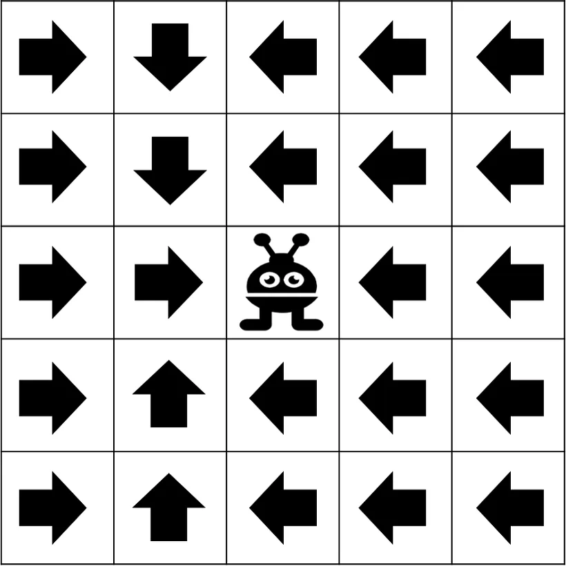
With a policy, the agent knows what to do in every state. But what we want from reinforcement learning is not just any policy—it is an optimal policy.

Reinforcement learning improves the current policy in pursuit of an optimal one.

Summary

We have used MDP to define a sequential decision-making problem. The agent chooses an action based on the rewards it expects to receive from its current state onward. The environment then supplies the actual reward and the next state. Repeating this process reveals errors in the agent's expectations. The expected future reward is called the 가치함수(Value Function), which we will discuss in the next chapter. The agent changes its value function and policy based on the rewards it actually receives. With enough learning, it can find a policy that yields the greatest reward.