DDIM: Denoising Diffusion Implicit Models

DDPM teaches a generative Markov chain that removes noise gradually. Sequential sampling needs many steps and is much slower than single-pass GANs. DDIM generalizes that process into a non-Markovian one.

DDIM: Denoising Diffusion ImplicitModels

paper: https://arxiv.org/abs/2006.11239 github: https://github.com/ermongroup/ddim

0. Abstract

DDPM generates high-quality images without adversarial training, but requires a long Markov chain and many sampling steps.

Denoising diffusion implicit models (DDIM) accelerate sampling by generalizing DDPM to non-Markovian diffusion. This enables a more deterministic generative process and high-quality samples ten to fifty times faster.

1. Introduction

Deep generative models have demonstrated high-quality generation across image domains. GANs outperform likelihood-based VAEs and flows in quality, but stable training restricts architectures and optimization, and they fail to cover all distribution modes.

DDPM and noise-conditional score networks produce GAN-quality samples without adversarial training by denoising through a generative Markov chain. Many iterations make them much slower than single-pass GANs.

To narrow this efficiency gap, DDIM uses the same training objective as DDPM but generalizes the forward process to non-Markovian chains. This can improve sampling efficiency ten to one hundred times with only a small quality loss.

DDIM also offers stronger consistency: samples starting from the same latent have similar high-level features. This enables semantically meaningful interpolation.

2. Background

If all conditionals are Gaussian with learnable means and fixed variances, DDPM's objective simplifies as follows.

Let $\epsilon_\theta := \{ \epsilon_\theta^{(t)} \}_{t=1}^T$ be a collection of $T$ functions. Each timestep-indexed $\epsilon_\theta^{(t)} : \mathcal{X} \rightarrow \mathcal{X}$ depends on trainable parameters $\theta^{(t)}$ and positive-coefficient vector $\gamma := [\gamma_1,...,\gamma_T]$, whose coefficients depend on $\alpha_{1:T}$. DDPM optimizes objective $\gamma = 1$ for generation performance. To generate $x_0$, sample $x_T$ from prior $p_\theta(x_T)$, then repeatedly sample $x_{t-1}$.

Forward-process length T is an important hyperparameter. Larger T makes reverse transitions closer to Gaussian and improves their approximation. DDPM therefore uses large T, such as 1,000. But these T steps are sequential, not parallel,$x_0$ making sampling slower than other generative models.

3. Variational Inference for Non-Markovian Forward Process

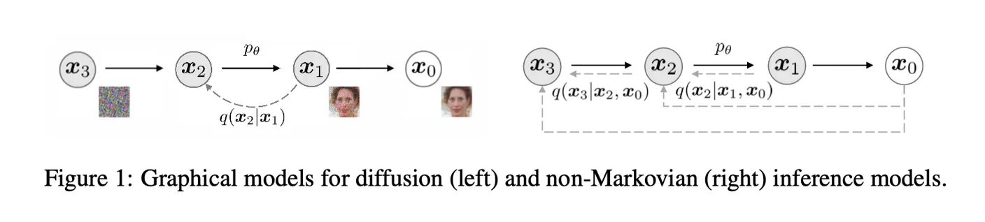
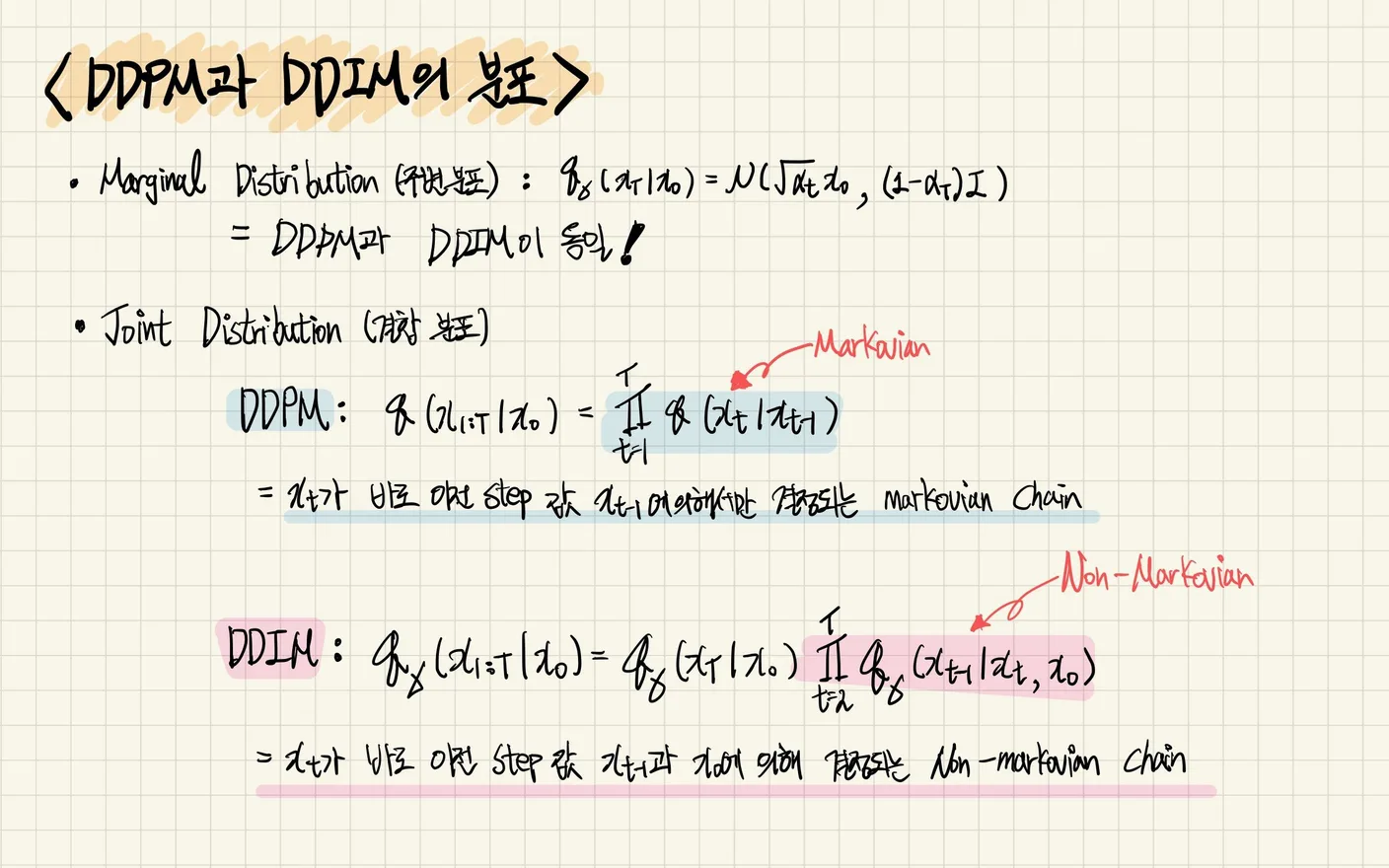
Reconsidering inference, the authors find that objective $L_\gamma$ depends only on marginal distributions $q(x_t|x_0)$, not directly on joint distribution $q(x_{1:T}|x_0)$. Many joints share those marginals, allowing a new non-Markovian process, shown on Figure 1's right. They establish this for Gaussian cases.

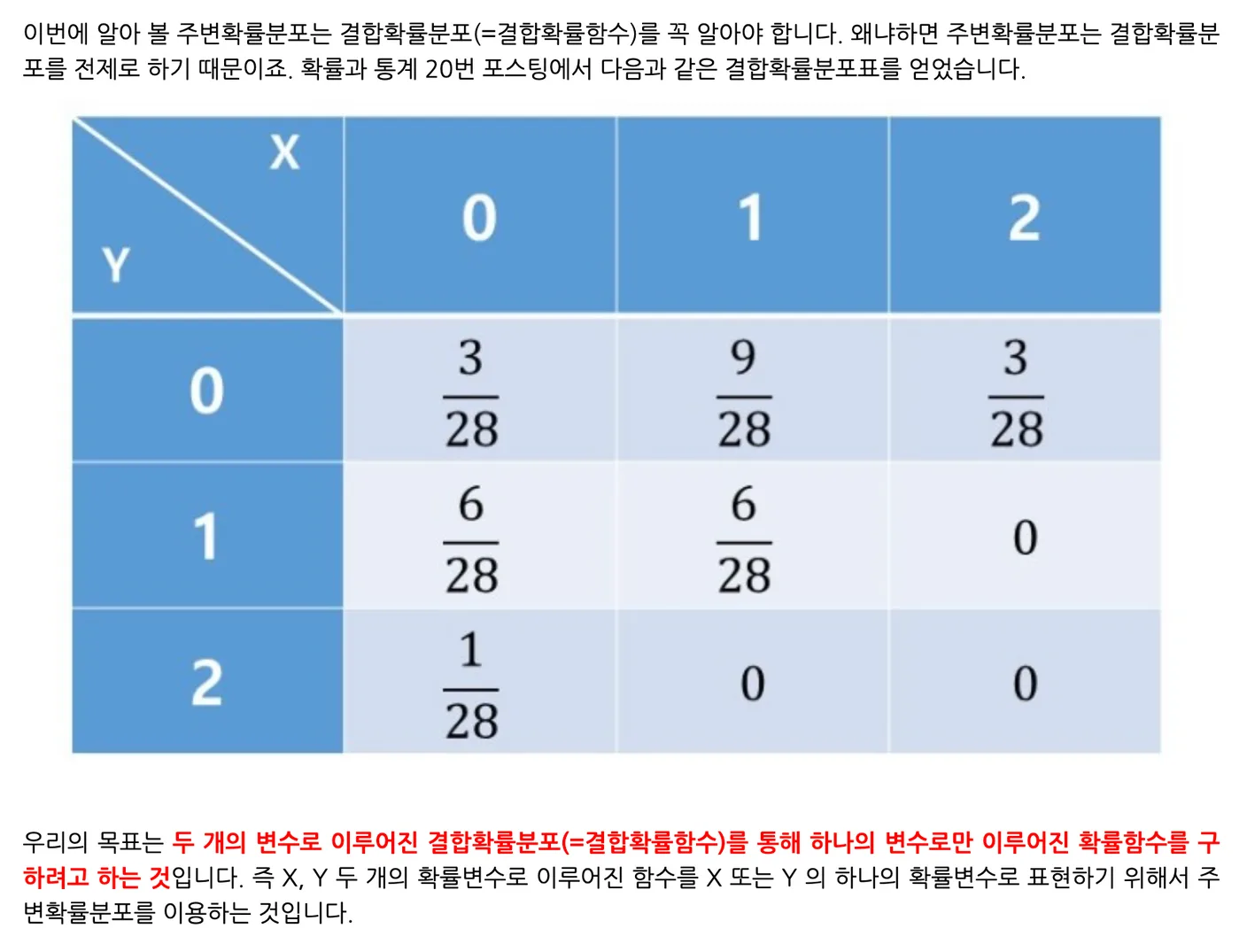
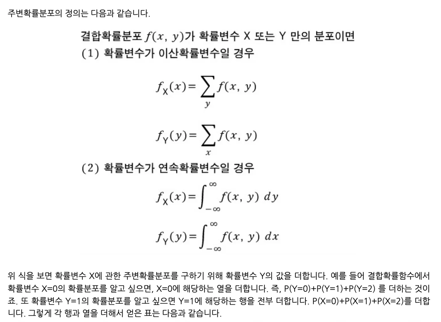
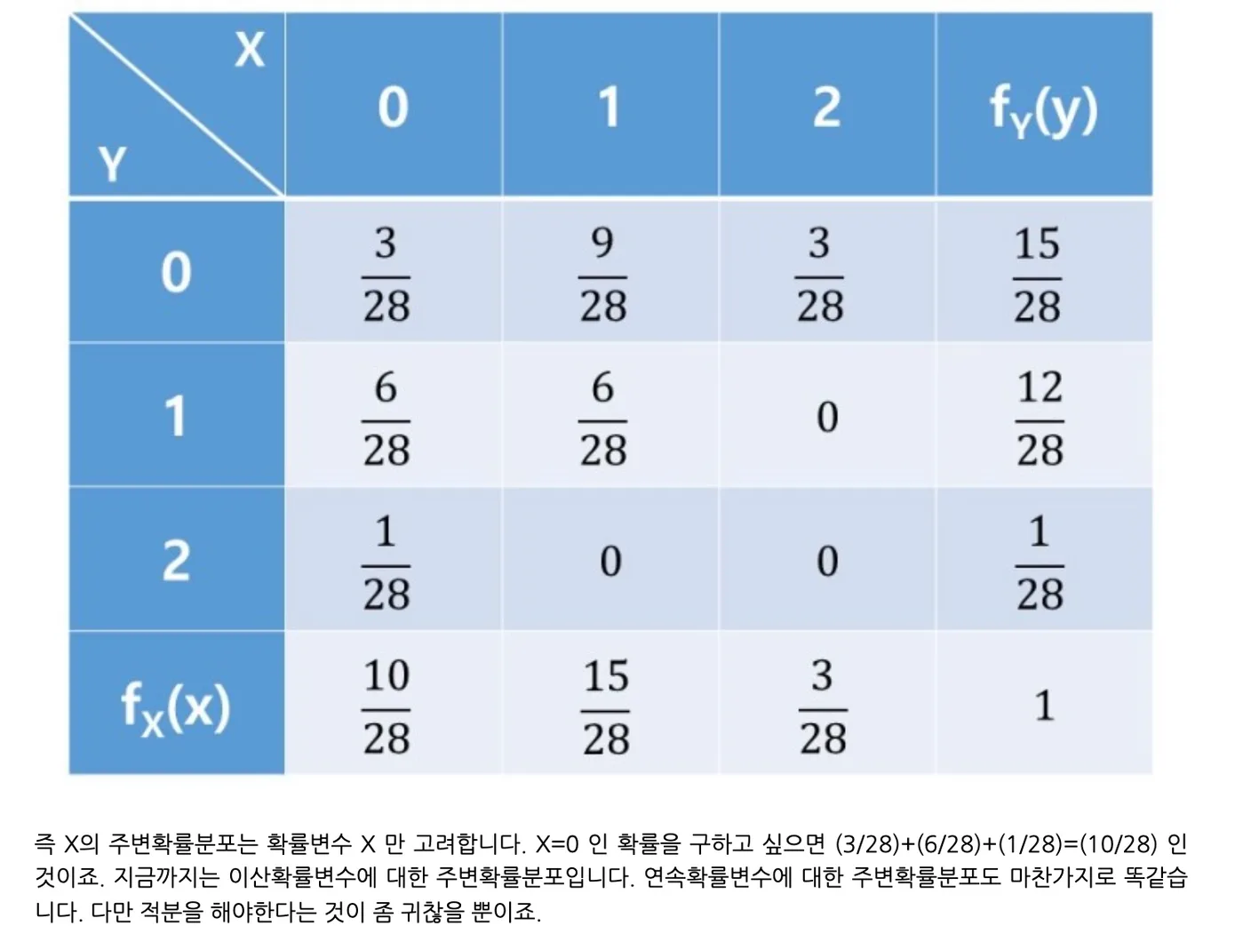
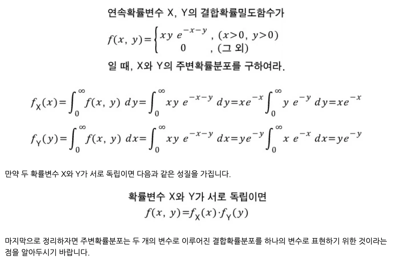
Definitions of joint and marginal distributions

📎

https://blog.naver.com/mykepzzang/220837645914

 

3.1. Non-Markovian Forward Process

To satisfy these equations, the forward inference mean must be:

The mean ensures $q_\sigma(x_t|x_0) = \mathcal{N}(\sqrt{\alpha_t}x_0, (1-\alpha_t)I)$ at every t, so the joint distribution has the desired marginals. Bayes' rule gives the following forward process.

Unlike DDPM, DDIM's forward process is no longer Markovian, because $x_t$ depends on both $x_{t-1}$ and $x_0$. $\sigma$ controls forward-process stochasticity. As it approaches zero,$x_{t-1}$ becomes fixed and deterministic.

3.2. Generative Process and Unified Variational Inference Objective

Next define learnable $p_\theta(x_{0:T})$. $p_\theta^{(t)}(x_{t-1}|x_t)$ uses known reverse conditional $q_\sigma(x_{t-1} |x_{t}, x_0)$ to sample $x_{t-1}$ from noisy $x_t$ using $x_0$. Intuitively, for observation $x_t$, first predict corresponding $x_0$, then sample $x_{t-1}$ through $q_\sigma(x_{t-1} |x_{t}, x_0)$.

Given $x_0 \sim q(x_0)$ and $\epsilon_t \sim \mathcal{N}(0,I)$, $x_t = \sqrt{\alpha_t}x_0 + \sqrt{1-\alpha_t}\epsilon$ Equation 4 gives $x_t$. Model $\epsilon_\theta^{(t)}(x_t)$ predicts $\epsilon_t$ from $x_t$ without knowing $x_0$. Rearranging for $x_0$ yields $x_0$'s prediction for $x_t$, the denoised observation. Fixed prior $p_\theta(x_T) = \mathcal{N}(0,I)$ then defines the generative process.

(1) denoised observation

• Expressing Equation 4 in terms of $x_0$

• Predicting $x_0$ with $x_t$

(2) generative process

• In $q_\sigma(x_{t-1}|x_t, \ f_\theta^{(t)}(x_t)$, denoised observation $f$ replaces $x_0$.

• Gaussian noise $\sigma_1^2I$ is added when $t=1$ to ensure a generative process.

(3) variational inference objective

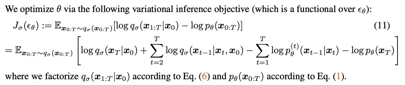
• Different choices of $\sigma$ yield different models.
• Setting $\sigma = 0$ gives the DDIM objective.
• Setting $\sigma ≠ 0$ gives the DDPM objective.

(4) Theorem 1.

• If $\gamma = 1$, the objective equals DDPM's variational lower bound.
• $L_1 = J_\sigma$

• Theorem 1 shows that $J_\sigma$ is a form of $L_\gamma$; $J_\sigma$ has its optimum when $\gamma=1$ ($L_1$).

4. Sampling from Generalized Generative Process

Since $\gamma=1$ gives the optimum, use $L_1$ as the objective.

Choosing $\sigma$ yields Markovian or non-Markovian processes. Regardless of $\sigma$, the parameters to learn are $\theta$.

• Thus, pretrained DDPM parameters$\theta$ can also be used in DDIM's generative process.

• Rather than introducing a new training method, DDIM generalizes diffusion to a non-Markovian chain and introduces a faster sampling method.

• A common approach is training with DDPM and sampling with DDIM, combining a strong model with fast generation.

4.1. Denoising Diffusion Implicit Model

In $p_\theta(x_{1:T})$, the equation below generates sample $x_{t-1}$ from $x_t$. $\epsilon_t \sim \mathcal{N}(0,I)$ is standard Gaussian noise independent of $x_t$, and $\alpha_0 := 1$ defines the setting. Different $\sigma$ yield different generative processes, but shared $\epsilon_\theta$ means no retraining.

4.2. Accelerated Generation Processes

Previously, generation approximated the reverse of a $T$-step forward process, requiring $T$ sampling steps. But denoising objective $L_1$, with $q_\sigma(x_t|x_0)$ fixed, no longer depends on that forward trajectory. We can consider fewer than $T$ steps, accelerating generation without training another model.

Suppose the forward process is defined not over all latents $x_{1:T}$, but a subset$\{x_{\tau_1},..., x_{\tau_{S}}\}$. $\tau$ is an increasing subsequence of $[1,…,T]$ of length S. Define its transitions so $q(x_{\tau_i}|x_0)$ matches the marginals.

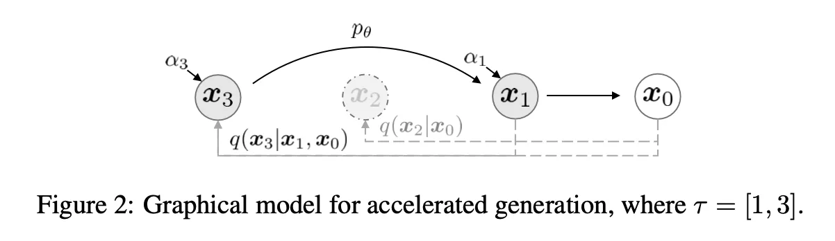
Generation samples in reverse$\tau$. This is the sampling trajectory. If the trajectory is shorter than $T$, computational efficiency improves substantially.

Small changes to Equation 12 yield a faster process applicable to DDPM and DDIM. Subsampled trajectories generate images faster, but if a model trains only at selected forward steps, generation can use only those steps; broader timestep training is needed.

• Training at many steps as in DDPM is more effective than training only selected steps in this interpretation of DDIM.

• Hence DDPM training with DDIM sampling is common.

4.3. Relevance to Neural ODEs

Rewriting DDIM iterations as Equation 12 makes their similarity to Euler integration for ordinary differential equations clearer.

To derive the ODE, reparameterize ($\sqrt{1-\alpha}/\sqrt{\alpha}$) with $\sigma$ and ($x/\sqrt{\alpha}$) with $\bar{x}$. When $\sigma(0) = 0$, Equation 13 becomes Euler's method for the ODE below.

With sufficiently fine discretization, reversing Equation 14's ODE enables encoding, reversing generation: $x_0$ → $x_T$.

5. Experiments

DDIM needs far fewer iterations than DDPM, giving ten- to one-hundred-fold speedups. With initial latent $x_T$ fixed, different trajectories preserve high-level features, and latent interpolation becomes possible.

DDIM can encode samples and reconstruct images from latents, unlike DDPM's stochastic process. Each dataset uses the same trained model with $T=1000$ and objective $L_1$. Only how samples are produced changes.

Experiments vary subsequences $\tau$ of $[ 1, ... , T ]$ and variance hyperparameter $\sigma$. $\eta \in \mathbb{R}_{\ge0}$ is directly controllable.

• If $\eta=1$: DDPM.

• If $\eta=0$: DDIM.

5.1. Sample Quality and Efficiency

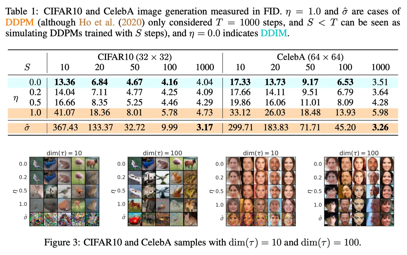
• Figure 3 reports FID for models trained on CIFAR-10 and CelebA.

• Quality improves as $dim(\tau)$ increases, trading off against computation. For the same $dim(\tau)$, DDIM performs better.

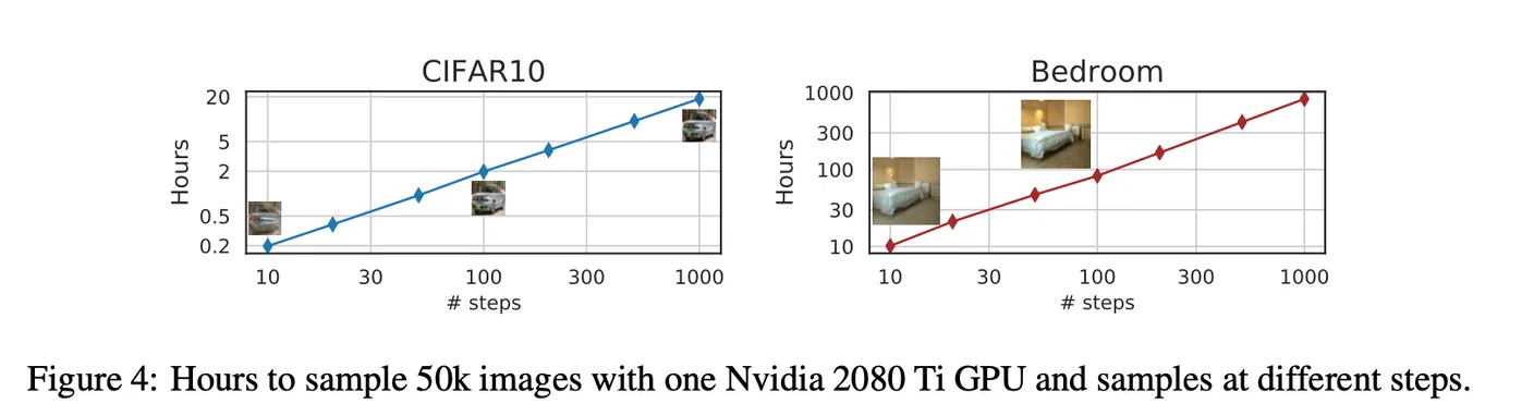
• Runtime rises linearly with trajectory length, showing that DDIM generates samples more efficiently.

• Quality requiring around 1,000 DDPM steps takes only 20–100 DDIM steps, ten to fifty times faster than DDPM.

5.2. Sample Consistency in DDIMs

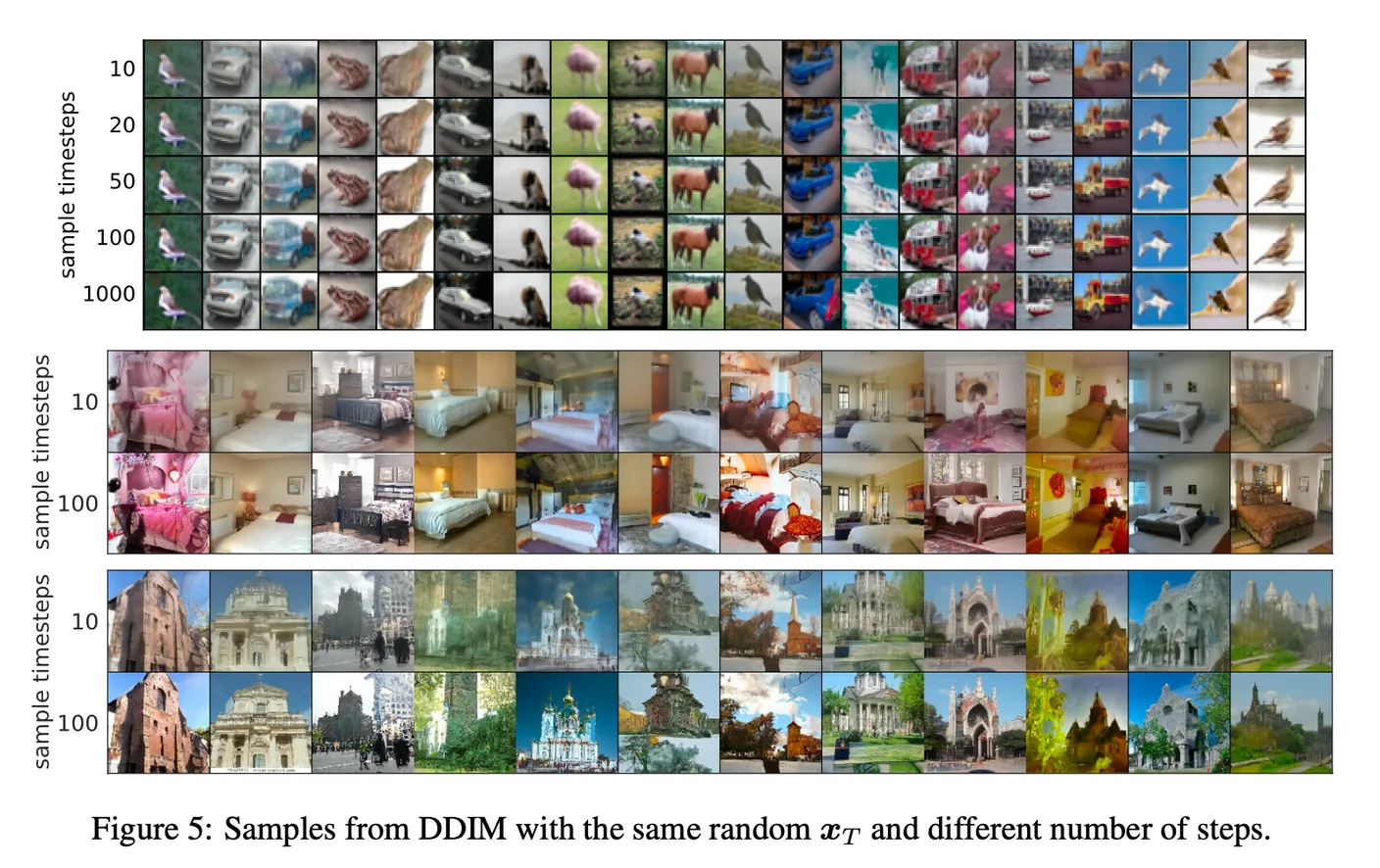
• DDIM generation is deterministic, and $x_0$ depends only on initial state $x_T$. Figure 5 compares trajectories for the same $x_T$; the same initial$x_T$ preserves similar high-level features.

• Thus, $x_T$ alone is an informative latent image encoding.

• Longer trajectories improve quality without significantly changing high-level features.

5.3. Interpolation in Deterministic Generative Processes

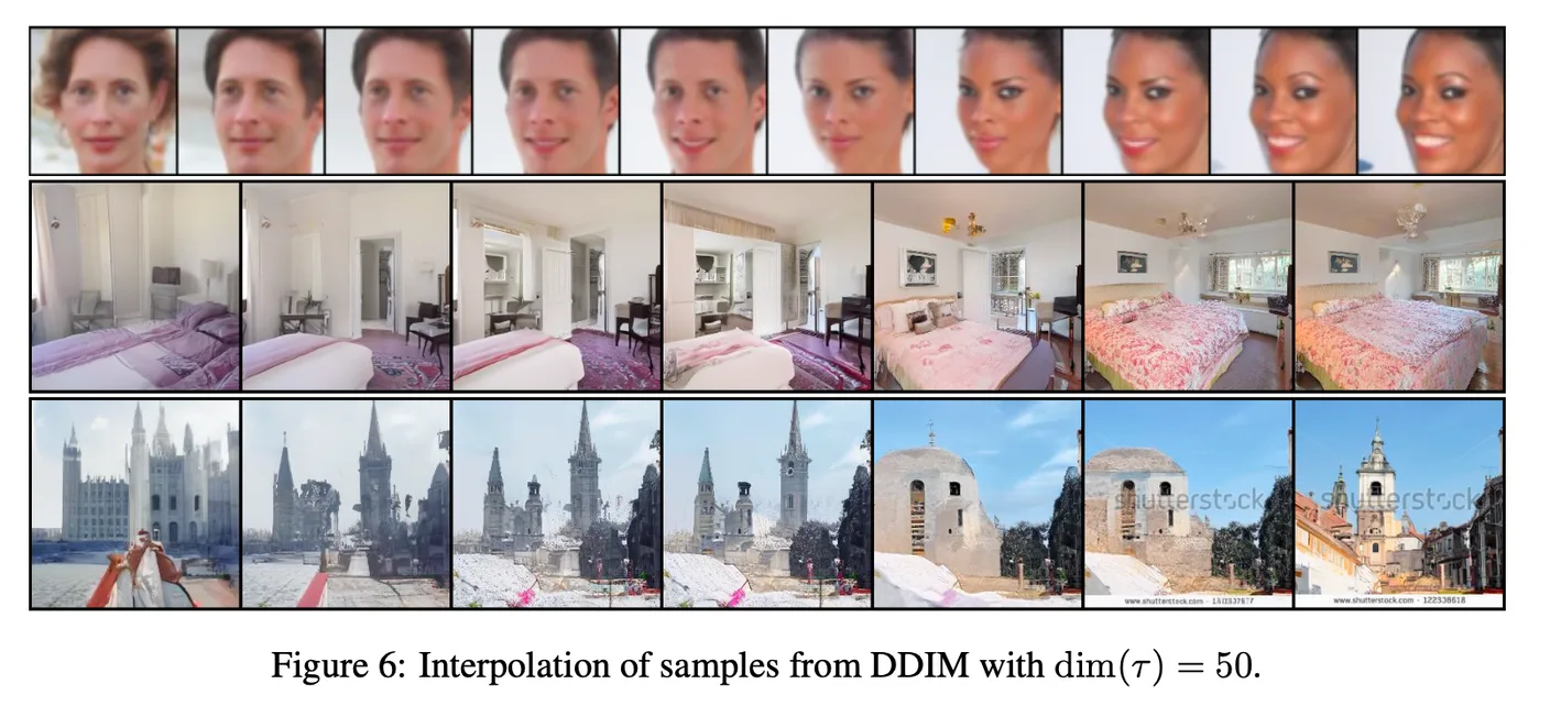
• Since $x_T$ encodes high-level features, the authors explore semantic interpolation, as in GANs, another implicit-model family. $x_T$Interpolation between two samples is possible.

• This is not possible in the same way with DDPM's stochastic generation.

5.4. Reconstruction from Latent Space

• DDIM's Euler-integrated ODE can encode $x_0$ into $x_T$ and reconstruct in reverse. As in neural ODEs, larger trajectory length $S$ lowers reconstruction error. DDPM does not offer the same reconstruction process.

Review

DDIM substantially improves DDPM sampling speed. Moving from Markovian to non-Markovian and stochastic to deterministic processes also enables interpolation, encoding, and reconstruction.

References

https://arxiv.org/abs/2010.02502

https://happy-jihye.github.io/diffusion/diffusion-2/