(3) Value Functions and Bellman Equations

This is the third review post in my series on Reinforcement Learning with Python and Keras.

http://www.yes24.com/Product/Goods/44136413

Chapter 2. Reinforcement Learning Basics I: Value Functions and Bellman Equations

We have defined the problem as MDP. The agent now uses MDP to find an optimal policy. Let us examine how. Warning: Equations ahead! ❗️

Value functions

How does an agent know which action is good? It must consider future rewards—but how can it consider rewards not yet received? 🧐 The concept associated with future rewards is 가치 함수.

We could simply sum all rewards from time t onward, giving $R_{t+1}+R_{t+2}+R_{t+3}+R_{t+4}+R_{t+5}+…$. But this creates three problems:

1. Present and future rewards are treated equally.

2. Receiving 100 once is indistinguishable from receiving 20 five times.

3. Over infinite time, receiving either 0.1 or 1 at every step gives an infinite sum.

Simple sums make it hard to judge the value of the state at time t. We therefore use 할인율, the discount factor introduced previously. The sum of future rewards expressed as values at time t is the 반환값, denoted $G_t$. Its equation follows.

A return sums rewards actually received during exploration. The book considers finite interactions only. Such a finite interaction is an 에피소드, with a terminal state—for example, the end of a chess game when the king is lost.

After an episode, a return answers 'How much reward did I receive from that point onward?' An episode from t = 1 to 5 gives five returns for the visited states.

Returns can differ between MDP episodes. The agent should therefore judge a state's value by the expected return, the concept of 가치함수, expressed below.

Rewards are stochastic, so their sum—the return—is a random variable. The value function, however, represents a particular quantity rather than a random variable, and uses lowercase notation. Substituting the return definition gives:

Although $R_{t+2}+\gamma R_{t+3} …$ is written as a return, it is not yet observed reward. It is expected future reward, which can also be expressed as a value function.

So far, the definition omits policy. But future rewards depend on it, since moving between states requires actions and the policy determines actions in every state.

Rewards depend on both state and action. Thus, the value function in an MDP depends on policy 정책. Writing the policy as a subscript makes this explicit.

This is the important 벨만 기대 방정식(Bellman Expectation Equation). It expresses the relationship between current-state value$v_\pi (s)$ and next-state value$v_\pi (S_{t+1})$.

Reinforcement learning is a story about how to solve Bellman equations. 🤧

Q-functions

A value function is a function, with inputs and outputs. The 상태 가치함수(state value-function) takes a state and returns the expected sum of future rewards. It tells the agent how good being in a state is.

What if a function gave the value of each action? The agent could choose directly from its values. A function measuring how good an action is in a state is 큐함수(Q Function), also called the action-value function.

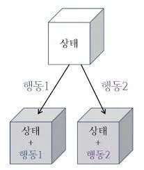
It takes state and action, written $q_\pi (s,a)$. Its relationship to the state-value function is:

1. Multiply each action's expected reward, Q-value $q_\pi (s,a)$, by its policy probability $\pi (a|s)$.

2. Sum Q-values weighted by $π(a|s)$ across all actions to obtain the state value.

Agents generally use the Q-function rather than state values as the basis for action selection. We will see why later. It also has a Bellman expectation equation, differing by conditioning on an action.

$q_\pi (s,a) = E_\pi [R_{t+1}+ \gamma q_\pi (S_{t+1}, A_{t+1})|S_t = s, A_t=a]$

The Bellman expectation equation

Now for Chapter 2's main dish, 벨만 기대 방정식. Listen closely! 👂🏻 It is called the expectation equation because it includes an expected value, expressing the relationship between current and next state values.

Why is this equation so important in reinforcement learning? 🤔 Revisit the value definition.

Calculating the expectation directly requires considering all future rewards, which is theoretically possible but very inefficient as the number of states increases. A computer needs another approach.

Suppose we need to add 1 one hundred times. One expression solves it as below.

Alternatively, define x and repeatedly add 1 to it.

X = 0
for i in range(100):
  X = X + 1

Bellman-based calculation follows the second approach: store a value and use a loop to approach the true value, updating the current estimate. How do we compute the expectation needed for each update?

It includes the probability of an action—the policy$\pi (a|s)$—and the probability of reaching a state after that action—the transition probability$P_{ss'}^a$. Include both in the calculation.

An example will help.

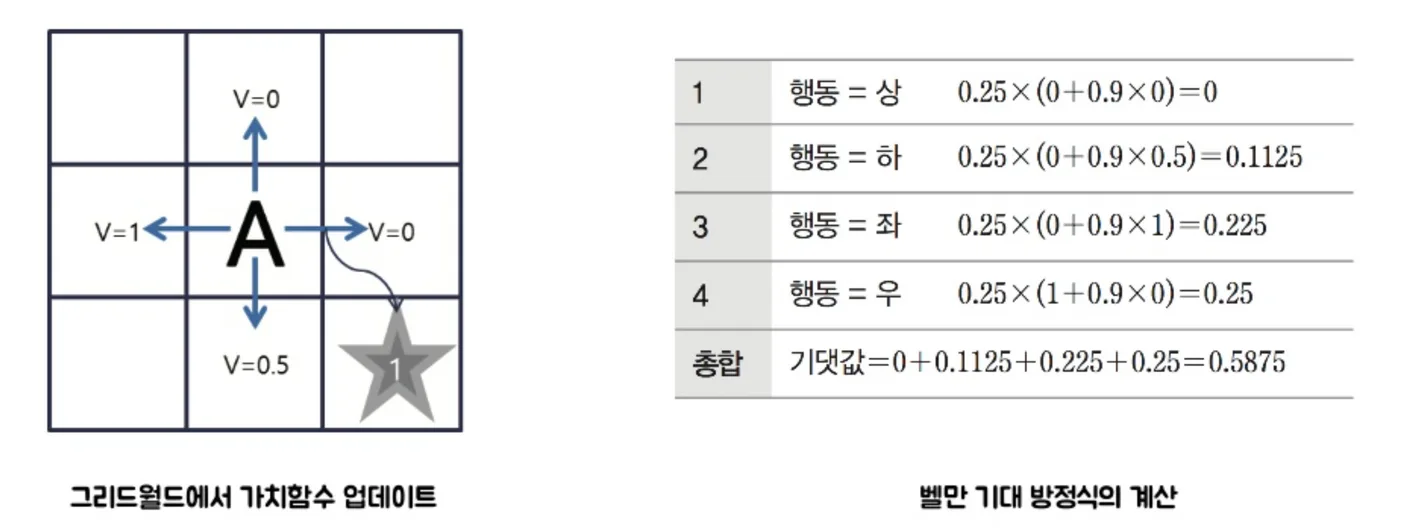
For simplicity:

1. Set 상태 변환 확률 ($P_{ss'}^a$) to 1: deciding to go left always moves left.

2. Use random 정책 ($π(a|s)$), selecting each action with 25% probability.

3. Set 할인율 ($γ$) to 0.9.

4. Let $s′$ be the state reached by the action, though it could generally be any state.

5. Gray stars represent rewards corresponding to $r(s,a)$.

Applying these assumptions rearranges the equation

into this form, allowing the calculations in the table above.

Repeated Bellman updates yield the true expected reward that the agent will receive.

The Bellman optimality equation

Initial values are arbitrary. Repeatedly calculating 벨만 기대 방정식 eventually makes both sides equal, assuming infinitely many repetitions. $v_\pi (s)$ converges, giving the true value function for current policy $π$.

Rearranging the expectation equation gives the true value function for the current policy. Dynamic programming will examine this in detail later.

But the true value function and optimal value function differ. ⭐️ 참 가치함수 is the true expected reward under a particular policy; 최적의 가치함수 is the value under the highest-reward policy among all policies.

We want an optimal policy, not merely current-policy values. We must update toward better policies. This raises two questions:

• How do we define a better policy?

• How do we judge which policy is better?

A better policy yields greater total reward, assessed through the value function. The policy with the greatest value across all policies is optimal. The optimal Q-function follows the same idea.

Suppose we have found optimal values. The optimal policy chooses the largest optimal Q-value in each state $s$. Knowing $q^∗$ is enough to derive it as below.

How do we find optimal Q-values? Doing so solves the sequential decision-making problem, or MDP. The next chapter addresses computation; here, we examine relationships between optimal values.

If the current state's value is optimal, the agent chooses the best action. Its selection criterion must be the optimal Q-function, giving this optimal-value equation.

Replacing Q-values with state values gives:

This is 벨만 최적 방정식(Bellman Optimality Equation), describing optimal state values. The Q-function version is:

It contains an expectation because transition probabilities determine the next state. 다이내믹 프로그래밍(Dynamic programming) uses these Bellman equations to solve an MDP by calculation, as the next chapter explains.

Summary

1. MDP: A mathematical definition of sequential decisions, comprising states $S_t$, actions $A_t$, rewards $r(s,a)$, transitions $P^a_{ss′}$, and discount factor $γ$.
$$v_\pi (s) = E_\pi [R_{t+1}+ \gamma v_\pi (S_{t+1})|S_t = s]$$

2. 가치함수: Expected total reward from the current state when following a policy.

3. 큐함수: Values actions and is used in policy updates.

1. 벨만 기대 방정식: Relates current and next-state values.
$$v_\pi (s) = E_\pi [R_{t+1}+ \gamma v_\pi (S_{t+1})|S_t = s]$$

2. 벨만 최적 방정식: Relates values under the optimal policy to next-state values.
$$v^*(s) = max_{a}E[R_{t+1} + \gamma v^*(S_{t+1}) | S_t=s, A_t=a]$$
 

Chapter 2 in one sentence

I should revisit the optimality equation and explain it more clearly. 🤥