ControlNet: Adding Conditional Control to Text-to-Image Diffusion Models

ControlNet: Adding Conditional Control to Text-to-Image Diffusion Models

paper: https://arxiv.org/abs/2302.05543 github: https://github.com/lllyasviel/ControlNet

0. Abstract

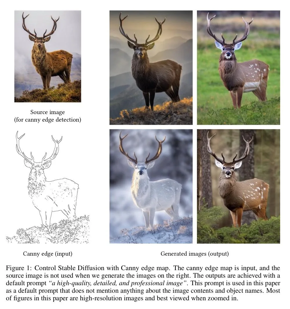
This paper introduces ControlNet, which controls a pretrained diffusion model such as Stable Diffusion using additional inputs: edge maps, segmentation maps, keypoints, and more. It learns task-specific conditions and trains robustly even on datasets smaller than 50,000 examples.

1. Introduction

After writing text to generate an image, we might ask:

1. Does text-prompt-based control adequately meet our need to generate the image we imagined?

2. What framework should we build to accommodate a wide range of task conditions and user controls, including inputs other than text?

3. Can we preserve a large model's capabilities learned from many images when adapting it to a specific task?

To answer these questions, the authors surveyed image-processing applications and made three observations, all pointing toward the need for less data and computation.

ControlNet is an end-to-end neural architecture that controls large image diffusion models such as Stable Diffusion with specific input conditions. It duplicates model weights into a trainable copy and a locked copy. The trainable copy learns conditional control from task-specific data, while the locked copy preserves the original capabilities. Special layers called zero convolutions connect the two blocks. Preserving production-ready weights makes training robust across dataset sizes. Because zero convolutions introduce no new noise, training is also as fast as fine-tuning the diffusion model.

Effects of a 1×1 convolution

• Reducing trainable parameters by changing channel counts

• Adding nonlinearity

• Computing object and positional information independently

3. Method

3.1. ControlNet

ControlNet manipulates the input conditions of neural network blocks to control the overall network's behavior. Such blocks include ResNet blocks, conv–BN–ReLU blocks, multi-head attention blocks, and transformer blocks.

For 2D features, given a feature map $x \in \mathbb{R}^{h\times w \times c}$, a neural network block $\mathcal{F}(\cdot \ ; \mathrm{\Theta})$, parameterized by $\Theta$, transforms $x$ into another feature map $y$.

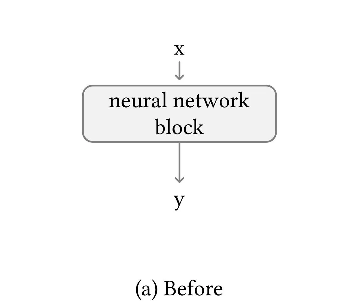
All parameters in $\Theta$ are locked and cloned into a trainable copy $\Theta_c$. The copied $\Theta_c$ is trained using an external condition vector $c$. The paper calls these the locked copy and trainable copy. Rather than directly updating the original weights, this preserves the quality learned from hundreds of millions of images and avoids overfitting on small datasets.

The blocks are connected by a special convolution layer $\mathcal{Z}(\cdot;\cdot)$, called a zero convolution: a 1×1 convolution whose weights and biases are initialized to zero. $\mathcal{Z}$ uses two parameter instances $\{\Theta_{z_1}, \Theta_{z_2}\}$, producing the ControlNet structure below.

A trained ControlNet recognizes the semantic content of its input conditions. In other words, it reflects the meaning of depth, normals, edges, and other conditions in generation.

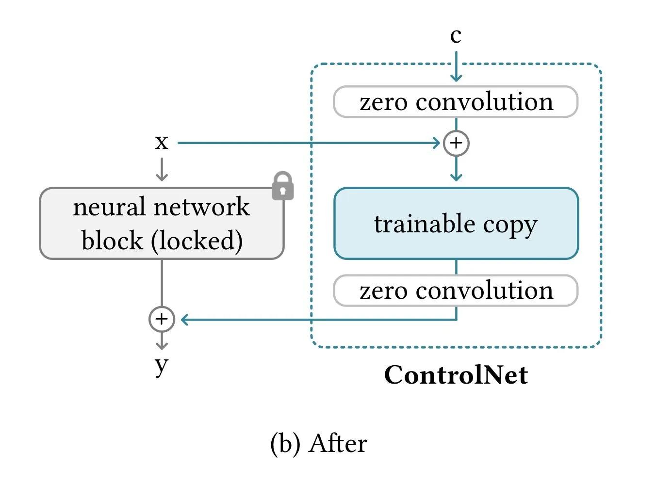
Because zero-convolution weights and biases start at zero, the first training step gives the following equations.

We can interpret them as follows.

These equations show that adding ControlNet does not affect the original network block before optimization. Its capabilities, functionality, and output quality remain intact. Subsequent optimization is as fast as fine-tuning, and much faster than training these layers from scratch.

Let us briefly examine gradients in a zero convolution. For a 1×1 convolution with weight $W$ and bias $B$, spatial position $h\times w$ denoted by $p$, and channel index $i$, the forward pass for an input map $I \in \mathbb{R}^{h\times w \times c}$ is as follows.

Before optimization, zero convolution has $W=0$ and $B=0$. Wherever $I_{p,i}$ is nonzero, its gradients are:

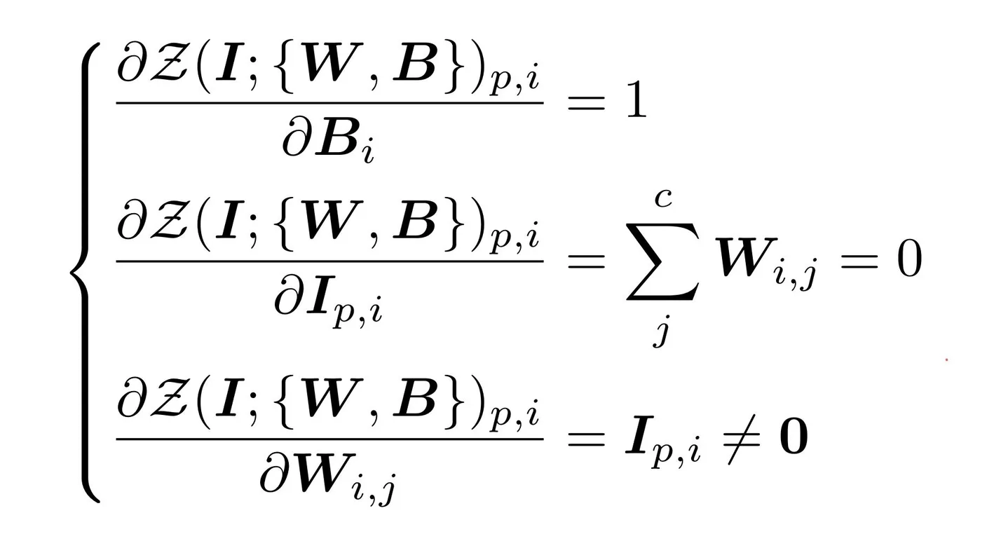
Although zero convolution can make the gradient for the feature term $I$ zero, the gradients for weight $W$ and bias $B$ are unaffected. At the first gradient-descent step, the weight $W$ becomes a nonzero matrix as long as the feature $I$ is nonzero. Simply put,$W$ even if $B$ are initialized to zero, $I$ only needs to be nonzero for learning to occur.

Thus, zero convolution becomes a distinctive connection layer that evolves from zero into optimized parameters.

3.2. ControlNet in Image Diffusion Model

Stable Diffusion is used as the example.

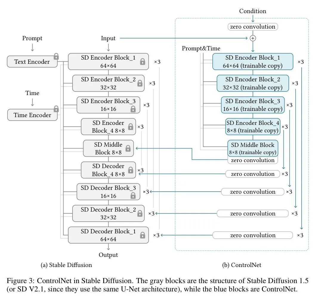
To stabilize training, Stable Diffusion preprocesses its 512×512 images into 64×64 latent images, similarly to VQ-GAN. ControlNet must likewise encode image-based conditions into a 64×64 feature space to match convolution sizes. The paper uses a small network $\mathcal{E}(\cdot)$, with 4×4 kernels and 2×2 strides, to encode an image-space condition $c_i$ into a feature map $c_f$.

The encoder transforms a 512×512 condition into a 64×64 feature map.

3.3. Training

Given a time step $t$, text prompt $c_t$, task-specific condition $c_f$, diffusion algorithm $\epsilon_\theta$, and noisy image $z_t$, the objective is as follows.

This objective can also be used directly for fine-tuning. During training, text prompts $c_t$ are randomly replaced with empty strings to improve recognition of the semantic content in the input condition maps.

4. Experiment

See the paper for further experimental results.

4.1. Experiment Setting

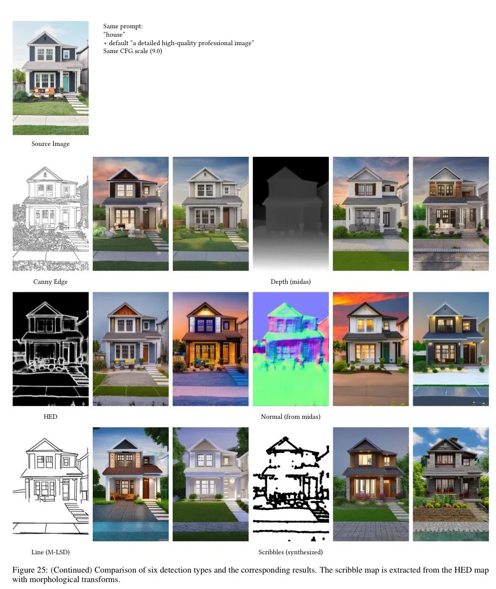
All experiments use CFG = 9.0, a DDIM sampler, and 20 steps. They test three prompt types: no prompt, a default prompt ('a professional, detailed, high-quality image'), and an automatic prompt.

5. Limitation

Reference

https://arxiv.org/abs/2302.05543